BIOSTATISTICS 1746 - Statistical Analysis of Clinical Trials Homework
VerifiedAdded on 2022/08/25
|11
|788
|46
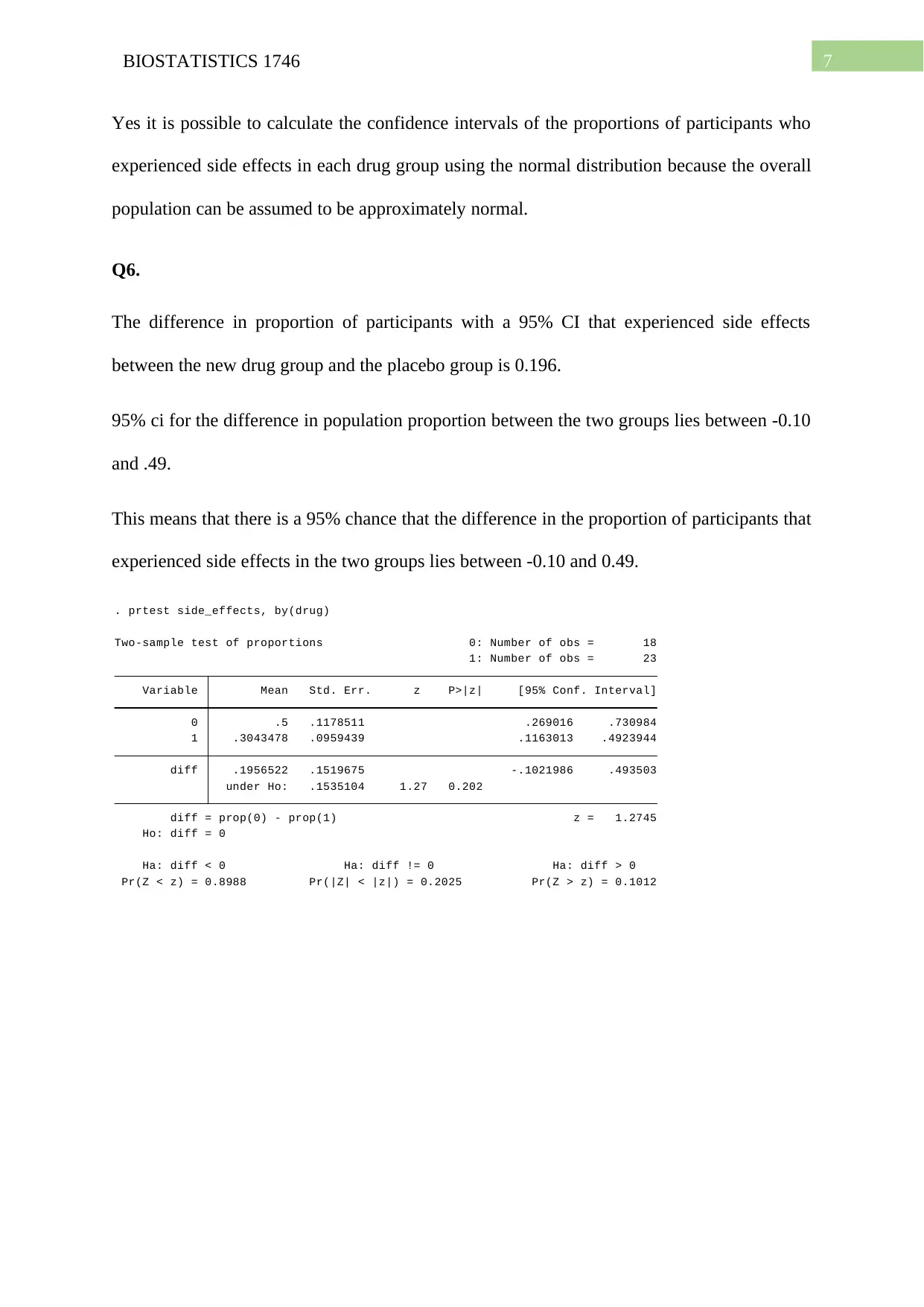
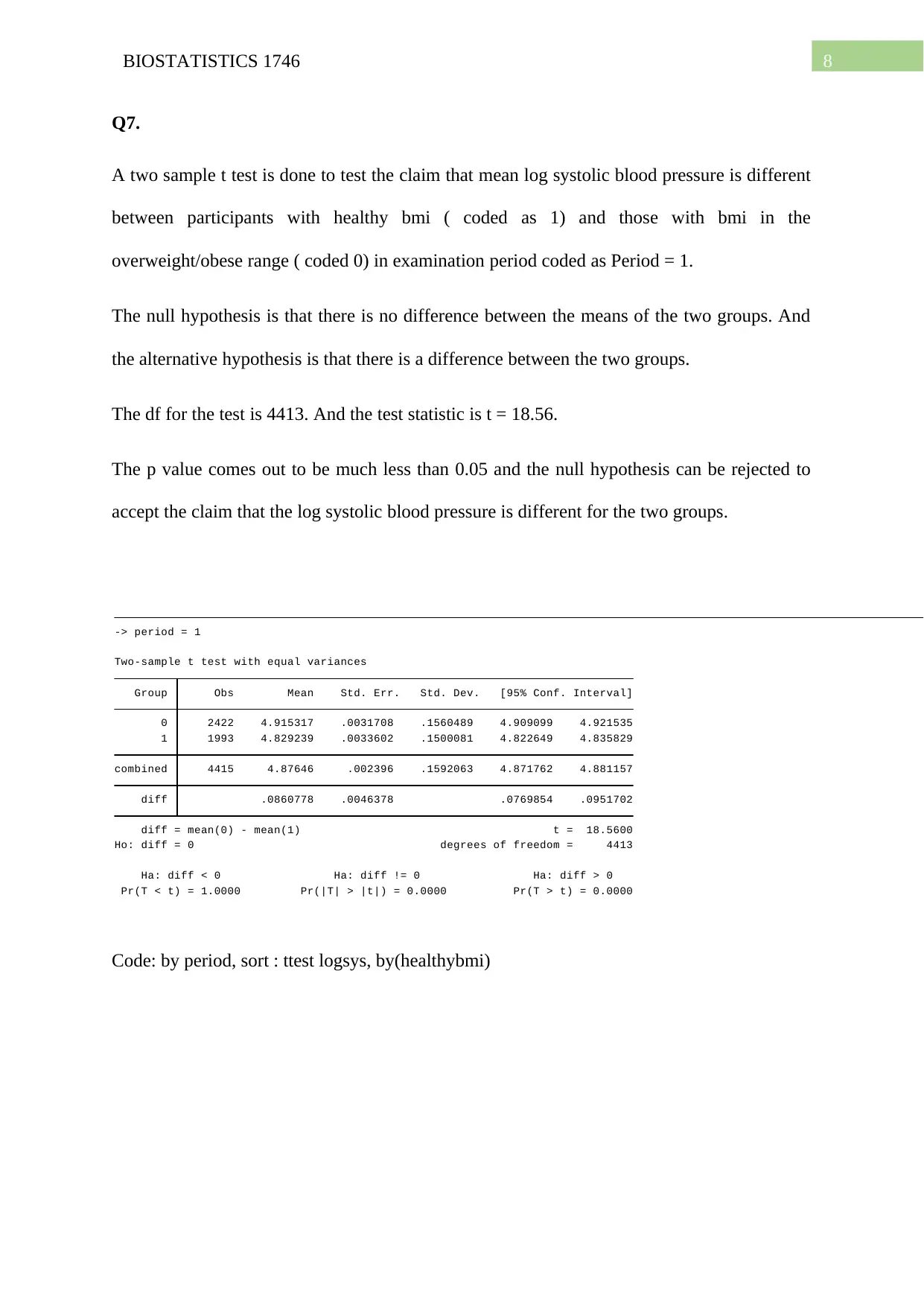
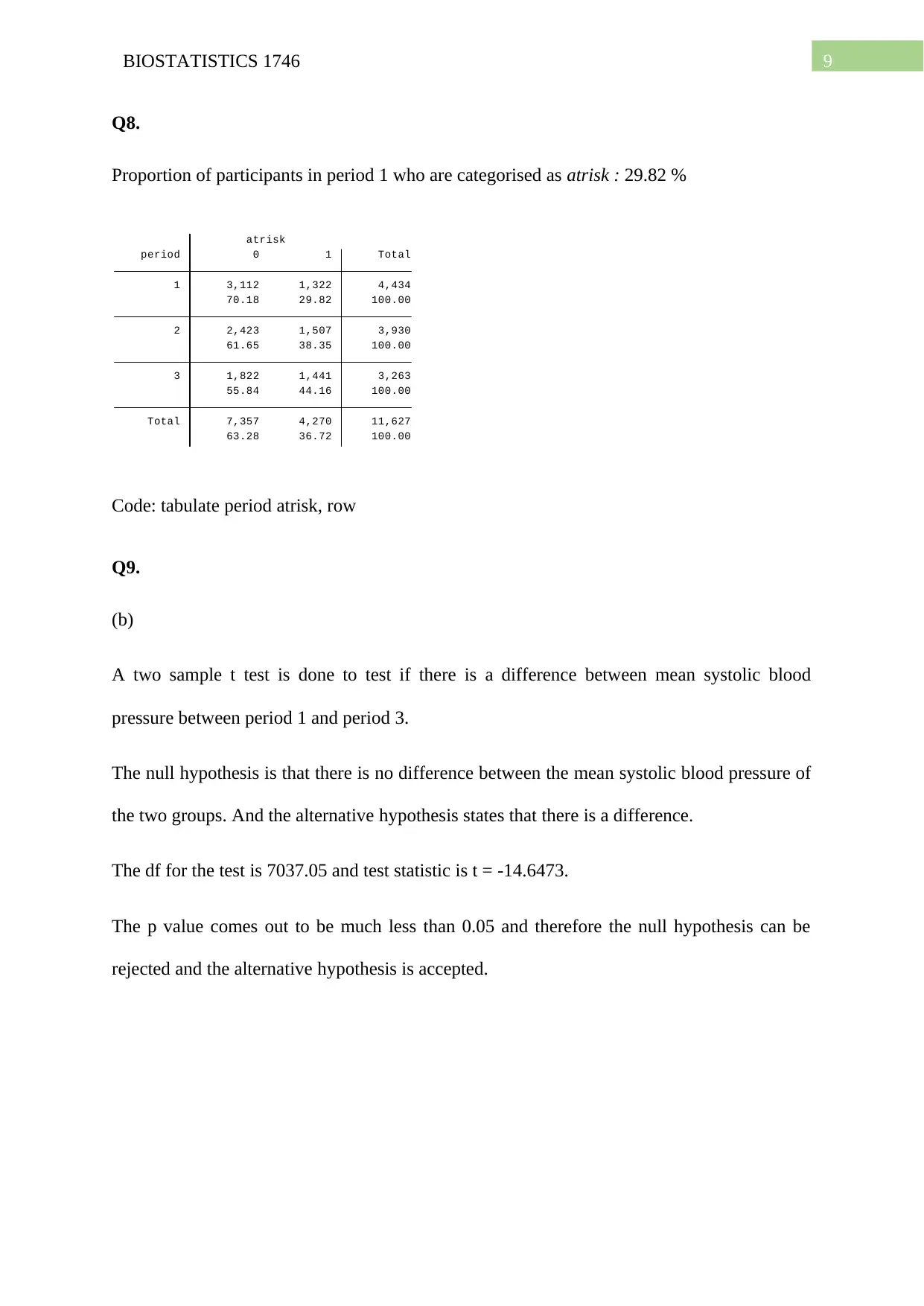
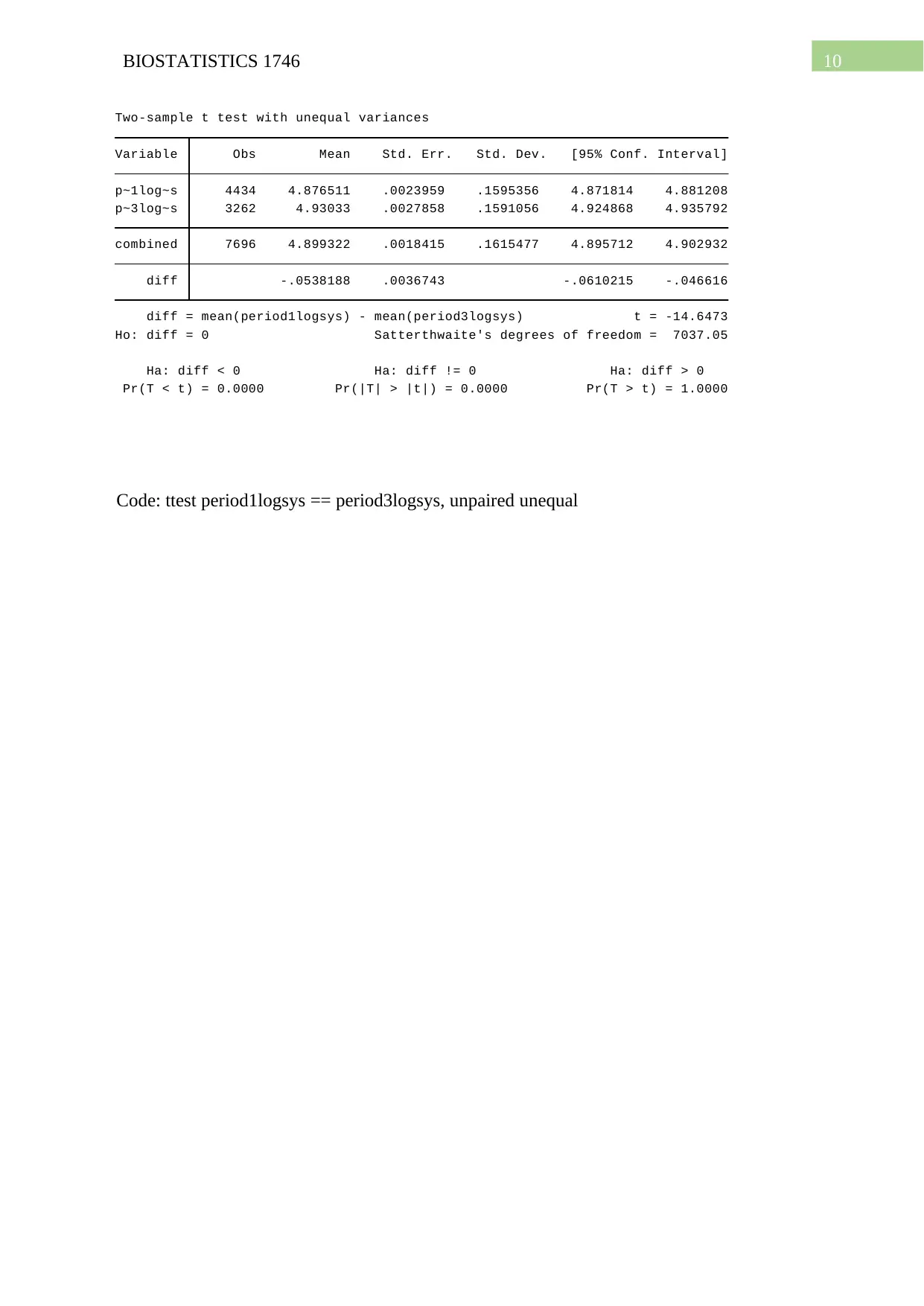
Homework Assignment
AI Summary
This biostatistics assignment solution presents a comprehensive analysis of clinical trial data. It includes calculations of range, IQR, and statistical tests like t-tests to compare the efficacy of a new drug against a placebo. The assignment explores the distribution of pain intensity scores, calculates confidence intervals, and examines the proportions of participants experiencing side effects. Furthermore, it investigates the relationship between health factors such as BMI and systolic blood pressure, performing t-tests to determine significant differences between groups. The solution utilizes Stata code to perform these analyses and includes relevant references. The assignment covers key concepts in biostatistics, including hypothesis testing, confidence intervals, and the interpretation of statistical results, providing a practical application of these concepts to real-world clinical trial data.


1 out of 11
Related Documents


Your All-in-One AI-Powered Toolkit for Academic Success.
+13062052269
info@desklib.com
Available 24*7 on WhatsApp / Email
![[object Object]](/_next/static/media/star-bottom.7253800d.svg)
Copyright © 2020–2026 A2Z Services. All Rights Reserved. Developed and managed by ZUCOL.