Curtin University MPH406 Epidemiology: Biostatistics Assignment 2
VerifiedAdded on 2023/06/03
|13
|4077
|433
Homework Assignment
AI Summary
This assignment from Curtin University's MPH406 Epidemiology & Biostatistics course delves into the statistical analysis of health data. It examines the relationship between pulse rate, BMI, and gender, employing t-tests and multiple regression models to test hypotheses and account for potential effect modifiers. The assignment also explores predictors of obesity using a dataset with variables like age, gender, smoking status, alcohol consumption, socio-economic status, and physical activity. Exploratory analyses, including scatter plots and correlation coefficients, are used to assess the strength of associations between these variables and BMI. The goal is to understand the factors influencing pulse rate and BMI, providing insights into public health research methods. Desklib offers a platform for students to access similar assignments and resources to aid in their studies.
CURTIN UNIVERSITY
SCHOOL OF PUBLIC HEALTH
Epidemiology & Biostatistics
Epidemiology & Biostatistics (MPH406)
Index No. EPID6001 (EPID6002)
Assignment 2 Semester/Session 2, 2018
Declaration
As I type (sign) my name below, I declare that the submitted assignment is my own work and has
not previously been submitted for assessment. I have carried out the analyses, interpreted and
answered all questions in this assignment myself. This work complies with Curtin University rules
concerning plagiarism and copyright. I understand that all forms of plagiarism, cheating and
unauthorised collusion are regarded seriously by the University and could result in penalties
including failure and possible exclusion from the University. I have retained a copy of this
assignment for my own records.
__________________________ ______________________ _______________
Name & ID of student Signature of student Date
Note: electronic signature is accepted
Paraphrase This Document
Need a fresh take? Get an instant paraphrase of this document with our AI Paraphraser
Assignment 2: BIOSTATISTICS
(Total marks 50 - to be scaled to 25%)
Question ONE
(Total: 23 marks)
In a study a fictitious random sample (Assign2Pulse2018S2.dta) was obtained with information of
pulse rate, gender, smoke status, level of activity, and BMI measured for 80 subjects. One of the
aims for the study is to understand the difference in pulse rate between overweight and non-
overweight people, and subjects’ gender differences need to be accounted for as well. In this
question, you are given one continuous dependent variable Y (pulse) and two categorical
independent variables (gender and BMICat) as follows:
Table 1
Variable Description
pulse Pulse rate beat per minute
gender 1 = male, 2 = female
BMICat 1 = non-overweight, 2 =overweight
Your task is to investigate the relationship between pulse and BMICat using appropriate procedures
and techniques, accounting for gender in the analyses as a potential effect modifier. Use a
significance level α of 5%.
Hint:
You may find helpful to follow the instructions in Lab 1 for t test.
You may find helpful to follow the strategy for analyses given in Module B6 and
Computing Lab 6.
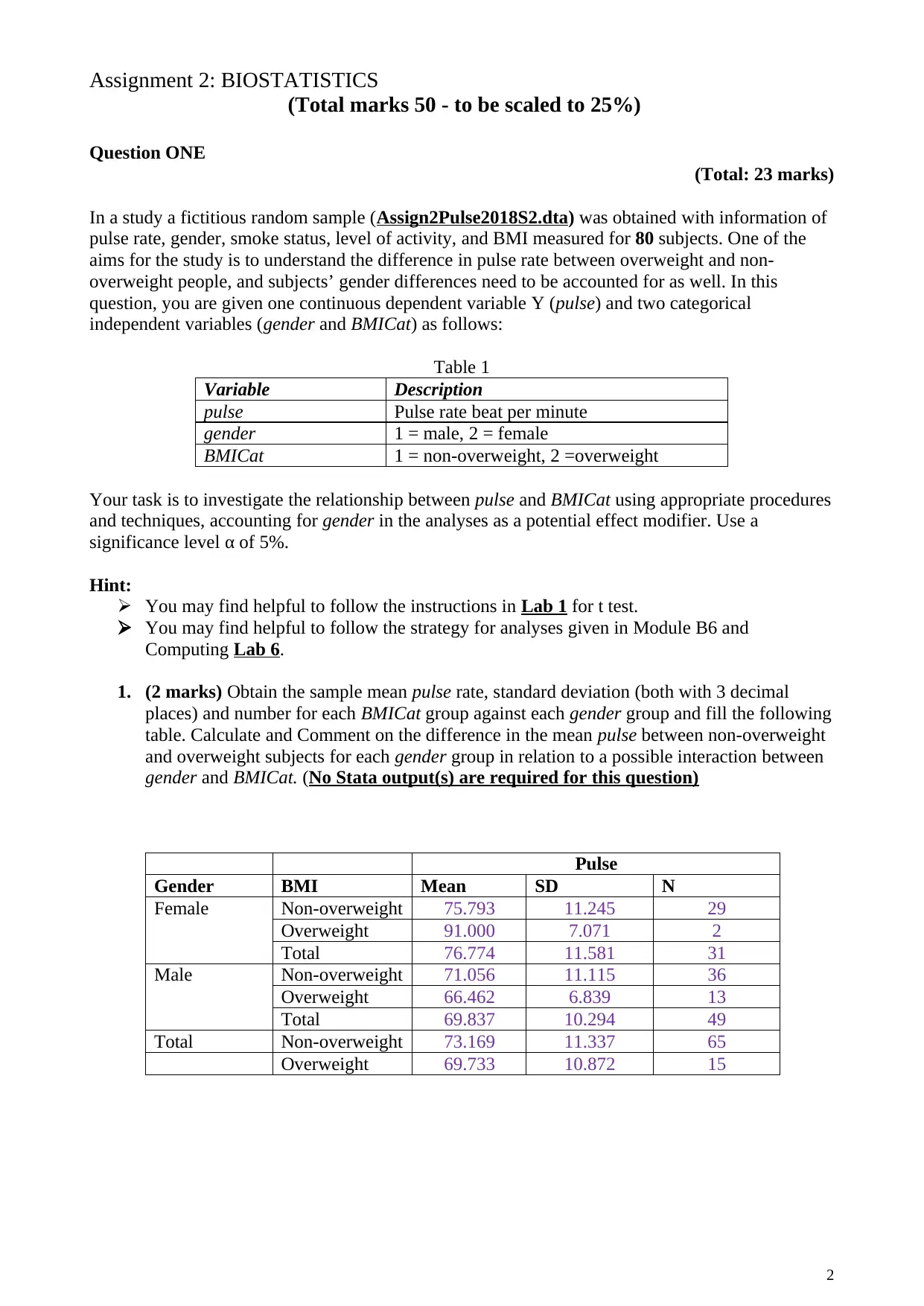
1. (2 marks) Obtain the sample mean pulse rate, standard deviation (both with 3 decimal
places) and number for each BMICat group against each gender group and fill the following
table. Calculate and Comment on the difference in the mean pulse between non-overweight
and overweight subjects for each gender group in relation to a possible interaction between
gender and BMICat. (No Stata output(s) are required for this question)
Pulse
Gender BMI Mean SD N
Female Non-overweight 75.793 11.245 29
Overweight 91.000 7.071 2
Total 76.774 11.581 31
Male Non-overweight 71.056 11.115 36
Overweight 66.462 6.839 13
Total 69.837 10.294 49
Total Non-overweight 73.169 11.337 65
Overweight 69.733 10.872 15
2
2. (4 marks) Test the hypothesis that the population mean pulse rate is the same for non-
overweight and overweight subjects.
(No Stata output(s) are required for this question)
i) Hypotheses: (1 mark)
HO: The average pulse rate is not significantly different for non-overweight and
overweight subjects.
HA: The average pulse rate is significantly different for non-overweight and
overweight subjects.
ii) Name the t test you used for the hypothesis (0.5 marks): Independent Samples t-test
iii) P value of the t test you used (0.5 marks): 0.2898
iv) Conclusion of the hypothesis test: (2 marks)
Since the p-value (0.2898) is greater than the 5% significance level, we fail to reject the
null hypothesis and conclude that the average pulse rate is not significantly different for
non-overweight and overweight subjects. That is, there is no significant evidence to
conclude that the average pulse rate for non-overweight and overweight subjects are
different.
3. (7 marks) Now assess the difference the population mean pulse rate between non-
overweight and overweight subjects using a multiple regression model, accounting for
gender in the analyses as a potential effect modifier.
i. Name the multiple regression model which is appropriate for this question. Why?
Linear regression; this is because the dependent variable (pulse rate) is continuous.
(1 mark)
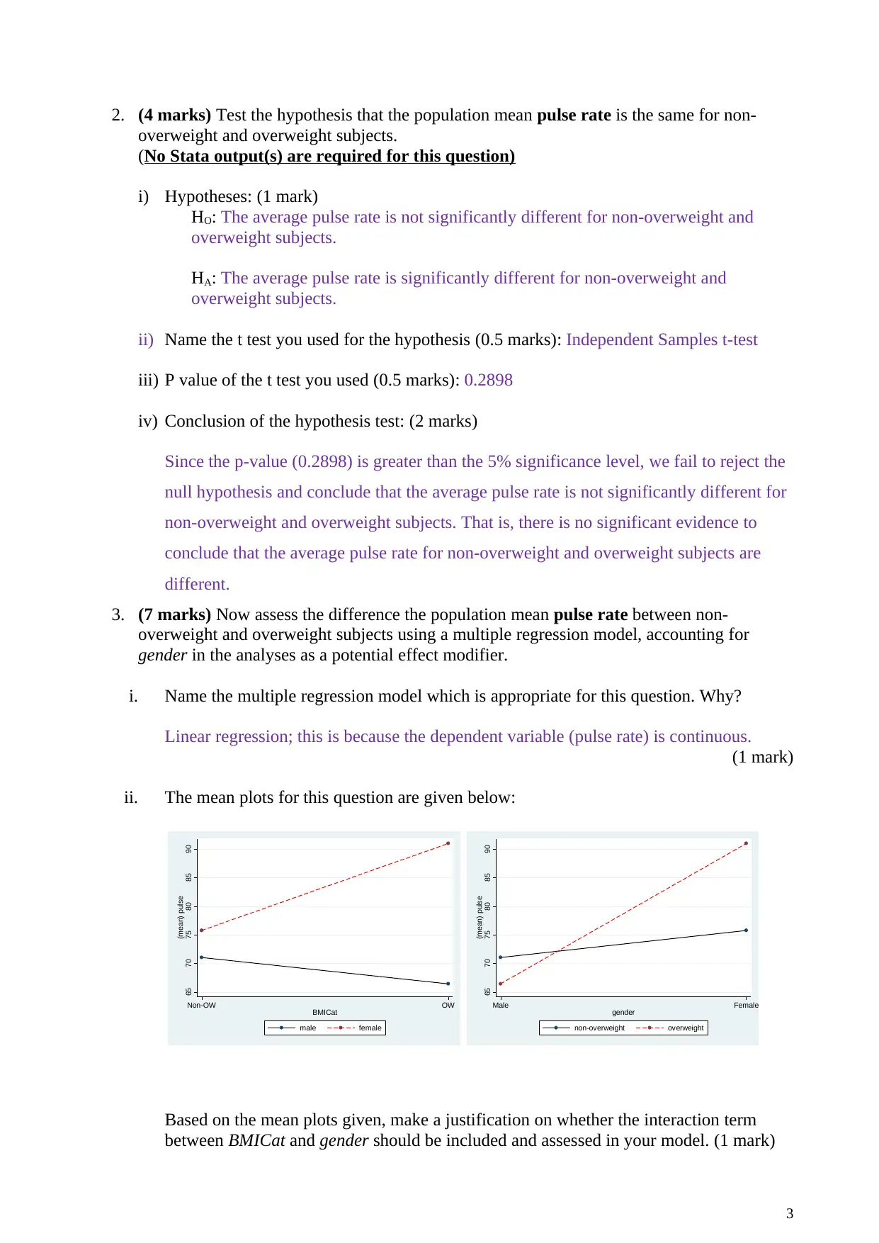
ii. The mean plots for this question are given below:
65 70 75 80 85 90
(mean) pulse
Non-OW OW
BMICat
male female
65 70 75 80 85 90
(mean) pulse
Male Female
gender
non-overweight overweight
Based on the mean plots given, make a justification on whether the interaction term
between BMICat and gender should be included and assessed in your model. (1 mark)
3
⊘ This is a preview!⊘
Do you want full access?
Subscribe today to unlock all pages.

Trusted by 1+ million students worldwide
The interaction term between BMICat and gender should be included and assessed in
the model since the interaction seems to be significant.
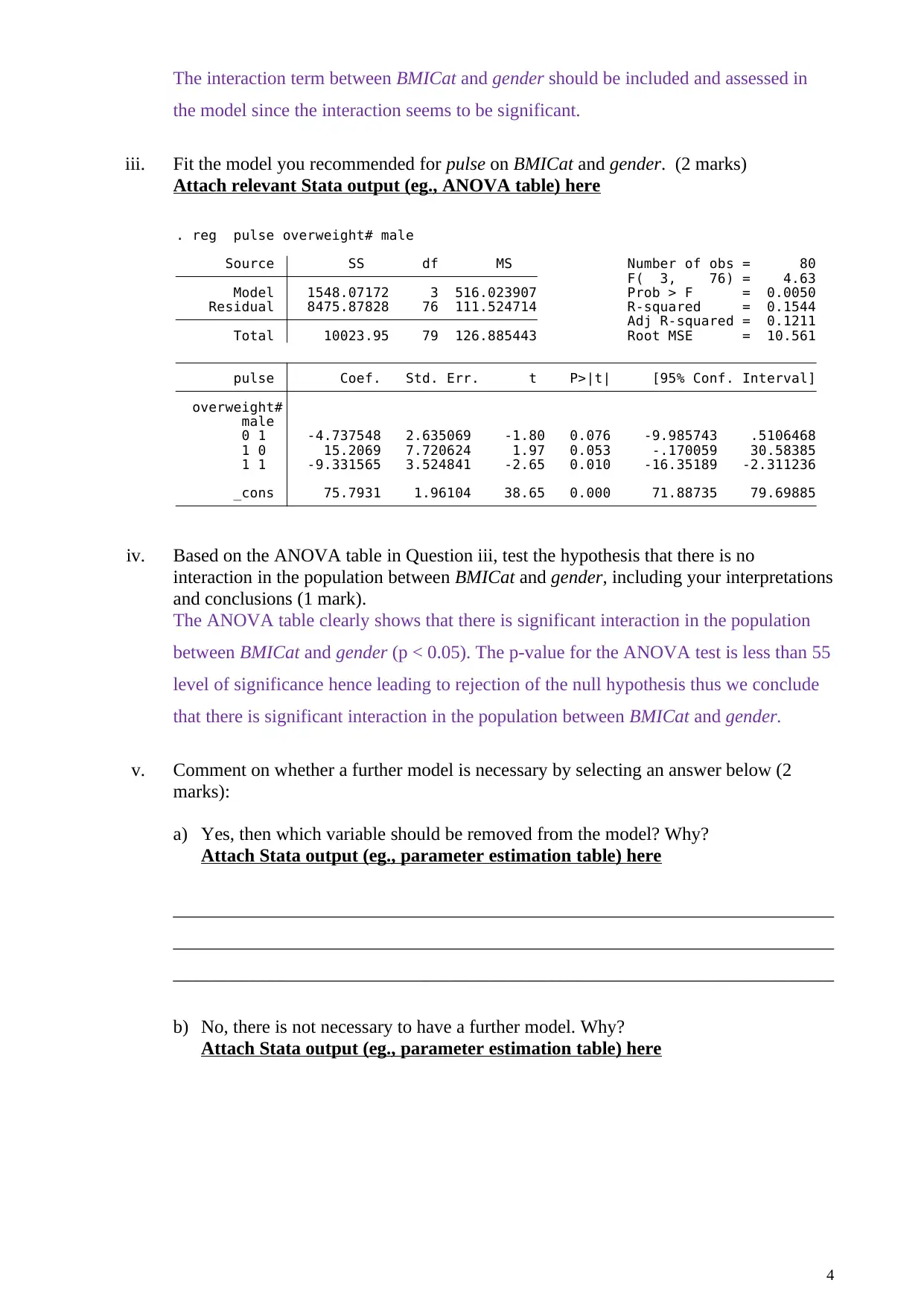
iii. Fit the model you recommended for pulse on BMICat and gender. (2 marks)
Attach relevant Stata output (eg., ANOVA table) here
_cons 75.7931 1.96104 38.65 0.000 71.88735 79.69885
1 1 -9.331565 3.524841 -2.65 0.010 -16.35189 -2.311236
1 0 15.2069 7.720624 1.97 0.053 -.170059 30.58385
0 1 -4.737548 2.635069 -1.80 0.076 -9.985743 .5106468
male
overweight#
pulse Coef. Std. Err. t P>|t| [95% Conf. Interval]
Total 10023.95 79 126.885443 Root MSE = 10.561
Adj R-squared = 0.1211
Residual 8475.87828 76 111.524714 R-squared = 0.1544
Model 1548.07172 3 516.023907 Prob > F = 0.0050
F( 3, 76) = 4.63
Source SS df MS Number of obs = 80
. reg pulse overweight# male
iv. Based on the ANOVA table in Question iii, test the hypothesis that there is no
interaction in the population between BMICat and gender, including your interpretations
and conclusions (1 mark).
The ANOVA table clearly shows that there is significant interaction in the population
between BMICat and gender (p < 0.05). The p-value for the ANOVA test is less than 55
level of significance hence leading to rejection of the null hypothesis thus we conclude
that there is significant interaction in the population between BMICat and gender.
v. Comment on whether a further model is necessary by selecting an answer below (2
marks):
a) Yes, then which variable should be removed from the model? Why?
Attach Stata output (eg., parameter estimation table) here
_______________________________________________________________________
_______________________________________________________________________
_______________________________________________________________________
b) No, there is not necessary to have a further model. Why?
Attach Stata output (eg., parameter estimation table) here
4
Paraphrase This Document
Need a fresh take? Get an instant paraphrase of this document with our AI Paraphraser
_cons 75.7931 1.96104 38.65 0.000 71.88735 79.69885
1 1 -9.331565 3.524841 -2.65 0.010 -16.35189 -2.311236
1 0 15.2069 7.720624 1.97 0.053 -.170059 30.58385
0 1 -4.737548 2.635069 -1.80 0.076 -9.985743 .5106468
male
overweight#
pulse Coef. Std. Err. t P>|t| [95% Conf. Interval]
Total 10023.95 79 126.885443 Root MSE = 10.561
Adj R-squared = 0.1211
Residual 8475.87828 76 111.524714 R-squared = 0.1544
Model 1548.07172 3 516.023907 Prob > F = 0.0050
F( 3, 76) = 4.63
Source SS df MS Number of obs = 80
. reg pulse overweight# male
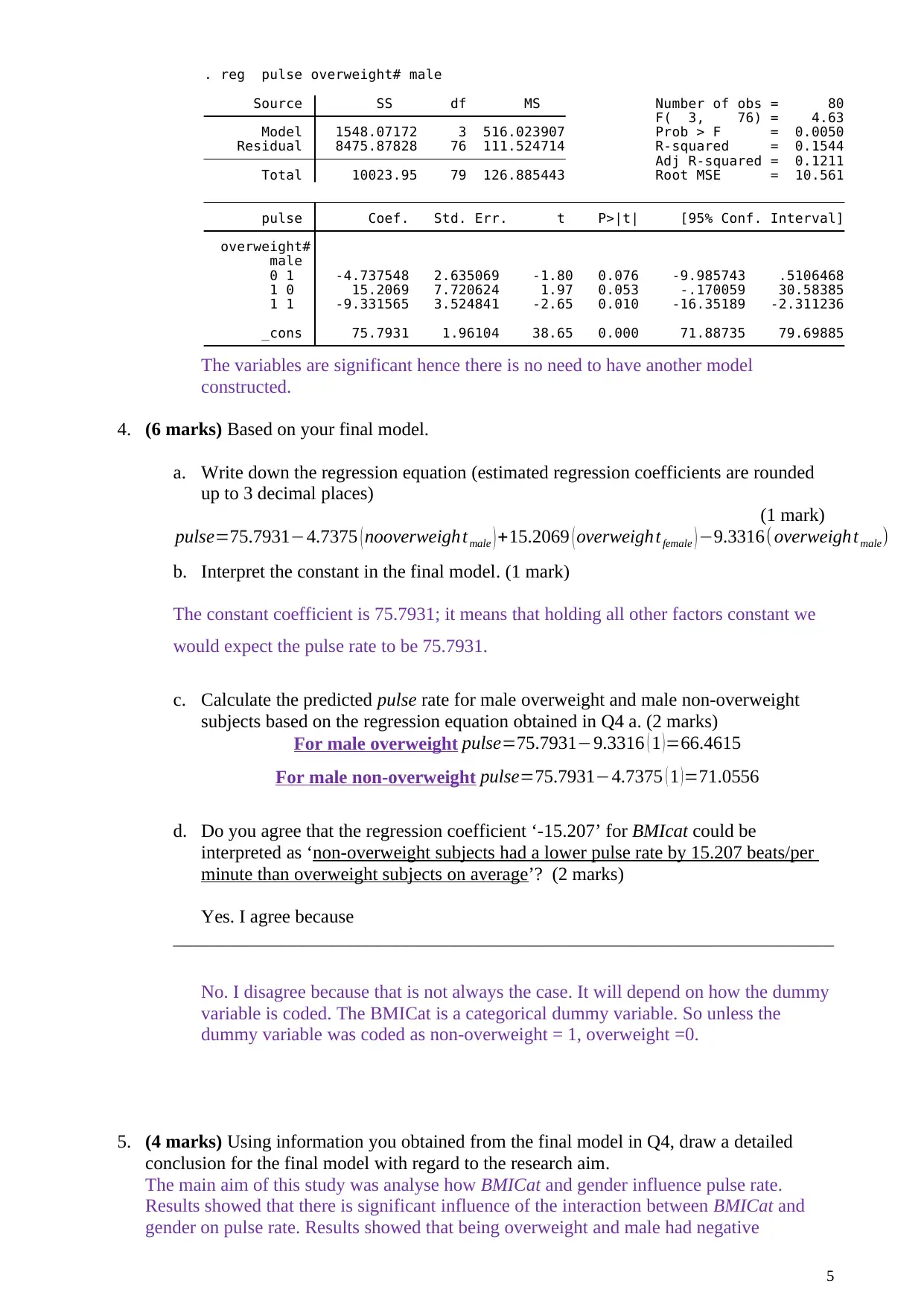
The variables are significant hence there is no need to have another model
constructed.
4. (6 marks) Based on your final model.
a. Write down the regression equation (estimated regression coefficients are rounded
up to 3 decimal places)
(1 mark)
pulse=75.7931−4.7375 ( nooverweigh tmale ) +15.2069 ( overweigh tfemale ) −9.3316( overweightmale)
b. Interpret the constant in the final model. (1 mark)
The constant coefficient is 75.7931; it means that holding all other factors constant we
would expect the pulse rate to be 75.7931.
c. Calculate the predicted pulse rate for male overweight and male non-overweight
subjects based on the regression equation obtained in Q4 a. (2 marks)
For male overweight pulse=75.7931−9.3316 ( 1 )=66.4615
For male non-overweight pulse=75.7931−4.7375 ( 1 )=71.0556
d. Do you agree that the regression coefficient ‘-15.207’ for BMIcat could be
interpreted as ‘non-overweight subjects had a lower pulse rate by 15.207 beats/per
minute than overweight subjects on average’? (2 marks)
Yes. I agree because
_______________________________________________________________________
No. I disagree because that is not always the case. It will depend on how the dummy
variable is coded. The BMICat is a categorical dummy variable. So unless the
dummy variable was coded as non-overweight = 1, overweight =0.
5. (4 marks) Using information you obtained from the final model in Q4, draw a detailed
conclusion for the final model with regard to the research aim.
The main aim of this study was analyse how BMICat and gender influence pulse rate.
Results showed that there is significant influence of the interaction between BMICat and
gender on pulse rate. Results showed that being overweight and male had negative
5
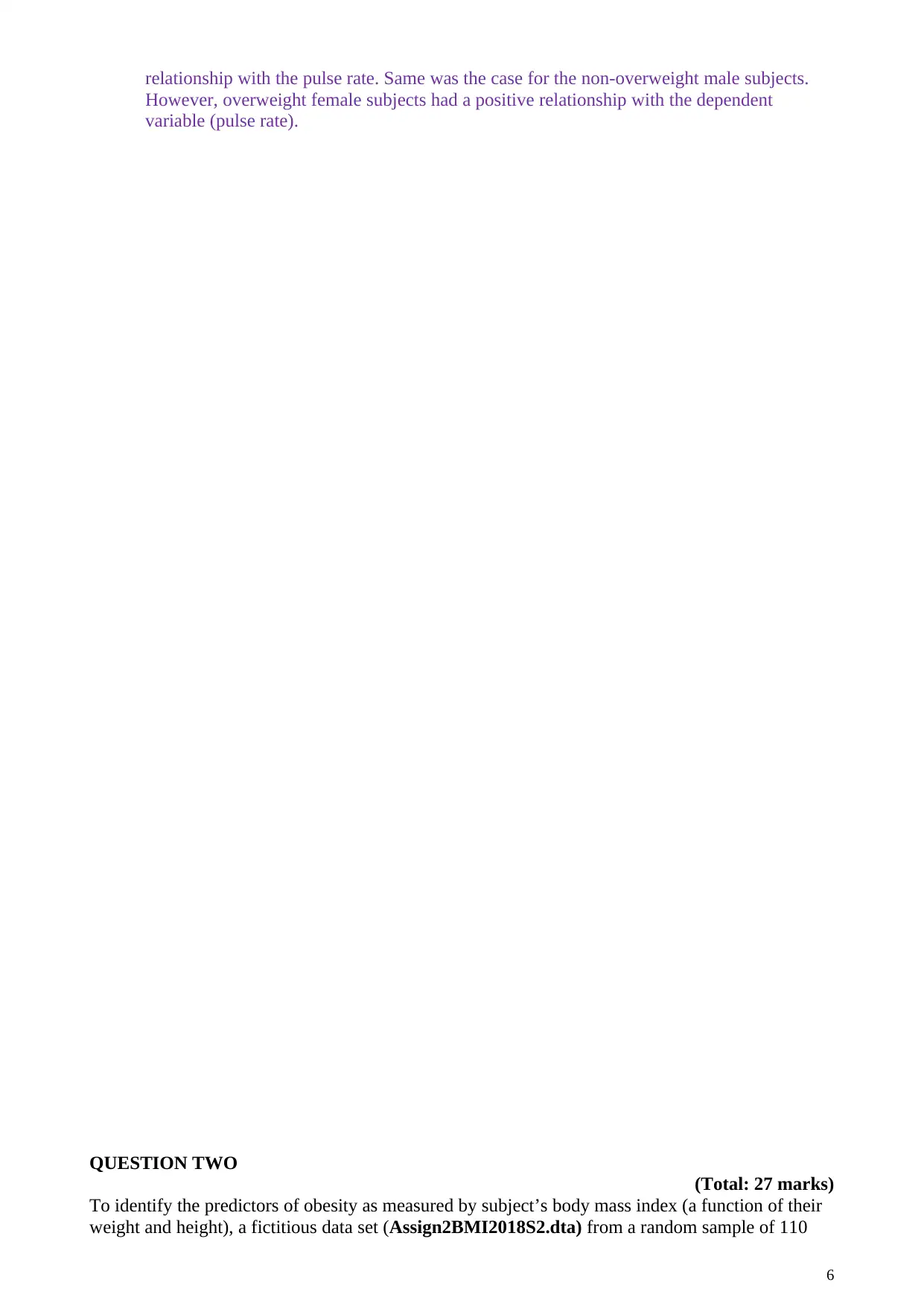
relationship with the pulse rate. Same was the case for the non-overweight male subjects.
However, overweight female subjects had a positive relationship with the dependent
variable (pulse rate).
QUESTION TWO
(Total: 27 marks)
To identify the predictors of obesity as measured by subject’s body mass index (a function of their
weight and height), a fictitious data set (Assign2BMI2018S2.dta) from a random sample of 110
6
⊘ This is a preview!⊘
Do you want full access?
Subscribe today to unlock all pages.

Trusted by 1+ million students worldwide
adults was used. The independent variables to be assessed are gender, smoking status, alcohol
consumption (grams of ethanol in a week), socio-economic status, whether the person regularly
participates in physical activity or not and subject’s age. The information of the variables is given
below in Table 1:
Table 1: Variables information
Variable Description
age The age of the participant (in years)
gender The gender of the participant: { 1 = Male , 2 = Female }
smoking Whether the person smokes or not: { 1 = Yes , 2 = No }
alcohol Alcohol consumption (grams of ethanol)
physact Whether the person regularly participates in physical activity:
{ 1 = Yes , 2 = No }
ses The socio-economic status of the participant:
{ 1 = Lower , 2 = Medium, 3 = Higher}
BMI Body mass index (in kg/m2)
You task is to investigate the relationship between BMI (dependent variable) and all the
independent variables given in the above table, using the appropriate procedures and techniques.
Hint:
i. You may find it helpful to follow the strategy for analyses given in Module B7 & B8 and
computing lab 8.
1. (7 marks) Exploratory analyses using descriptive statistics and plots.
1.1 Examine the linear relationship between BMI and age using scatter plot and Pearson’s
correlation coefficient. (1 mark)
(No Stata output(s) are required for this question)
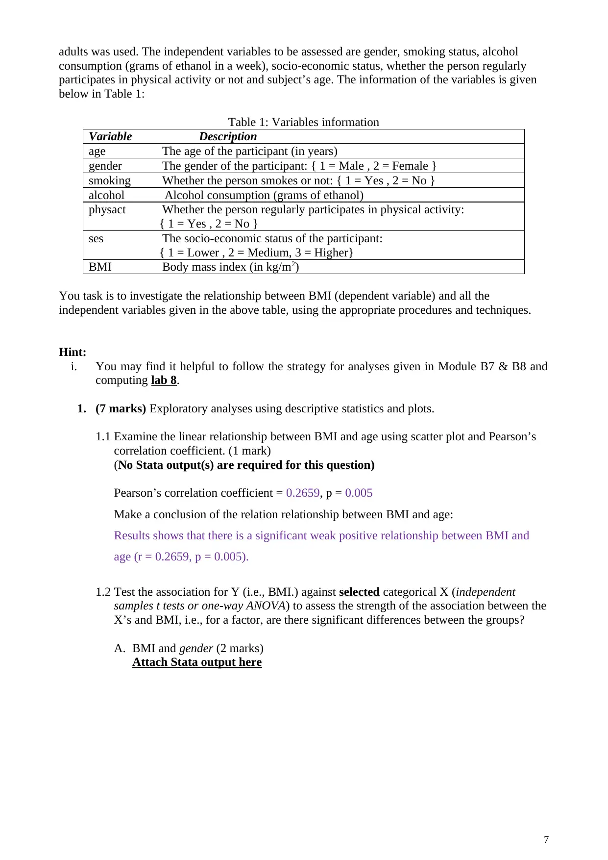
Pearson’s correlation coefficient = 0.2659, p = 0.005
Make a conclusion of the relation relationship between BMI and age:
Results shows that there is a significant weak positive relationship between BMI and
age (r = 0.2659, p = 0.005).
1.2 Test the association for Y (i.e., BMI.) against selected categorical X (independent
samples t tests or one-way ANOVA) to assess the strength of the association between the
X’s and BMI, i.e., for a factor, are there significant differences between the groups?
A. BMI and gender (2 marks)
Attach Stata output here
7
Paraphrase This Document
Need a fresh take? Get an instant paraphrase of this document with our AI Paraphraser
Pr(T < t) = 0.9382 Pr(|T| > |t|) = 0.1236 Pr(T > t) = 0.0618
Ha: diff < 0 Ha: diff != 0 Ha: diff > 0
Ho: diff = 0 degrees of freedom = 108
diff = mean(Male) - mean(Female) t = 1.5519
diff 1.08001 .6959173 -.2994192 2.459439
combined 110 24.70073 .3402765 3.56885 24.02631 25.37515
Female 68 24.28836 .3722574 3.069713 23.54533 25.03139
Male 42 25.36837 .6496067 4.209933 24.05646 26.68028
Group Obs Mean Std. Err. Std. Dev. [95% Conf. Interval]
Two-sample t test with equal variances
. ttest BMI, by( gender)
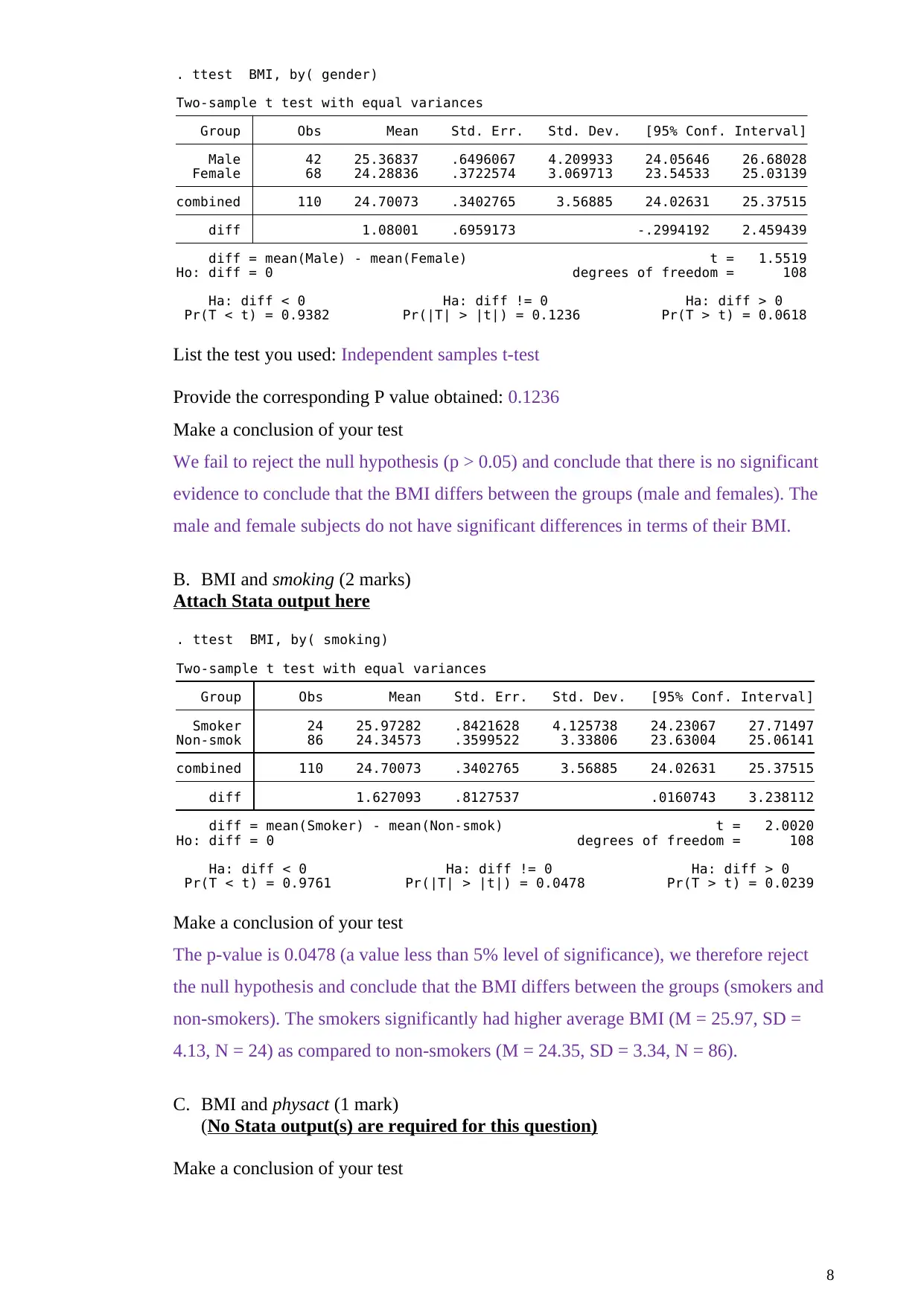
List the test you used: Independent samples t-test
Provide the corresponding P value obtained: 0.1236
Make a conclusion of your test
We fail to reject the null hypothesis (p > 0.05) and conclude that there is no significant
evidence to conclude that the BMI differs between the groups (male and females). The
male and female subjects do not have significant differences in terms of their BMI.
B. BMI and smoking (2 marks)
Attach Stata output here
Pr(T < t) = 0.9761 Pr(|T| > |t|) = 0.0478 Pr(T > t) = 0.0239
Ha: diff < 0 Ha: diff != 0 Ha: diff > 0
Ho: diff = 0 degrees of freedom = 108
diff = mean(Smoker) - mean(Non-smok) t = 2.0020
diff 1.627093 .8127537 .0160743 3.238112
combined 110 24.70073 .3402765 3.56885 24.02631 25.37515
Non-smok 86 24.34573 .3599522 3.33806 23.63004 25.06141
Smoker 24 25.97282 .8421628 4.125738 24.23067 27.71497
Group Obs Mean Std. Err. Std. Dev. [95% Conf. Interval]
Two-sample t test with equal variances
. ttest BMI, by( smoking)
Make a conclusion of your test
The p-value is 0.0478 (a value less than 5% level of significance), we therefore reject
the null hypothesis and conclude that the BMI differs between the groups (smokers and
non-smokers). The smokers significantly had higher average BMI (M = 25.97, SD =
4.13, N = 24) as compared to non-smokers (M = 24.35, SD = 3.34, N = 86).
C. BMI and physact (1 mark)
(No Stata output(s) are required for this question)
Make a conclusion of your test
8
Ha: diff < 0 Ha: diff != 0 Ha: diff > 0
Ho: diff = 0 degrees of freedom = 108
diff = mean(Male) - mean(Female) t = 1.5519
diff 1.08001 .6959173 -.2994192 2.459439
combined 110 24.70073 .3402765 3.56885 24.02631 25.37515
Female 68 24.28836 .3722574 3.069713 23.54533 25.03139
Male 42 25.36837 .6496067 4.209933 24.05646 26.68028
Group Obs Mean Std. Err. Std. Dev. [95% Conf. Interval]
Two-sample t test with equal variances
. ttest BMI, by( gender)
List the test you used: Independent samples t-test
Provide the corresponding P value obtained: 0.1236
Make a conclusion of your test
We fail to reject the null hypothesis (p > 0.05) and conclude that there is no significant
evidence to conclude that the BMI differs between the groups (male and females). The
male and female subjects do not have significant differences in terms of their BMI.
B. BMI and smoking (2 marks)
Attach Stata output here
Pr(T < t) = 0.9761 Pr(|T| > |t|) = 0.0478 Pr(T > t) = 0.0239
Ha: diff < 0 Ha: diff != 0 Ha: diff > 0
Ho: diff = 0 degrees of freedom = 108
diff = mean(Smoker) - mean(Non-smok) t = 2.0020
diff 1.627093 .8127537 .0160743 3.238112
combined 110 24.70073 .3402765 3.56885 24.02631 25.37515
Non-smok 86 24.34573 .3599522 3.33806 23.63004 25.06141
Smoker 24 25.97282 .8421628 4.125738 24.23067 27.71497
Group Obs Mean Std. Err. Std. Dev. [95% Conf. Interval]
Two-sample t test with equal variances
. ttest BMI, by( smoking)
Make a conclusion of your test
The p-value is 0.0478 (a value less than 5% level of significance), we therefore reject
the null hypothesis and conclude that the BMI differs between the groups (smokers and
non-smokers). The smokers significantly had higher average BMI (M = 25.97, SD =
4.13, N = 24) as compared to non-smokers (M = 24.35, SD = 3.34, N = 86).
C. BMI and physact (1 mark)
(No Stata output(s) are required for this question)
Make a conclusion of your test
8
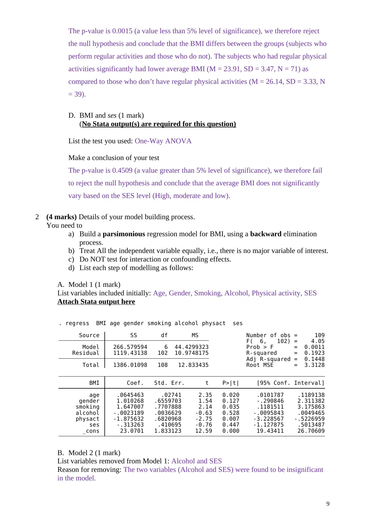
The p-value is 0.0015 (a value less than 5% level of significance), we therefore reject
the null hypothesis and conclude that the BMI differs between the groups (subjects who
perform regular activities and those who do not). The subjects who had regular physical
activities significantly had lower average BMI (M = 23.91, SD = 3.47, N = 71) as
compared to those who don’t have regular physical activities (M = 26.14, SD = 3.33, N
= 39).
D. BMI and ses (1 mark)
(No Stata output(s) are required for this question)
List the test you used: One-Way ANOVA
Make a conclusion of your test
The p-value is 0.4509 (a value greater than 5% level of significance), we therefore fail
to reject the null hypothesis and conclude that the average BMI does not significantly
vary based on the SES level (High, moderate and low).
2 (4 marks) Details of your model building process.
You need to
a) Build a parsimonious regression model for BMI, using a backward elimination
process.
b) Treat All the independent variable equally, i.e., there is no major variable of interest.
c) Do NOT test for interaction or confounding effects.
d) List each step of modelling as follows:
A. Model 1 (1 mark)
List variables included initially: Age, Gender, Smoking, Alcohol, Physical activity, SES
Attach Stata output here
_cons 23.0701 1.833123 12.59 0.000 19.43411 26.70609
ses -.313263 .410695 -0.76 0.447 -1.127875 .5013487
physact -1.875632 .6820968 -2.75 0.007 -3.228567 -.5226959
alcohol -.0023189 .0036629 -0.63 0.528 -.0095843 .0049465
smoking 1.647007 .7707888 2.14 0.035 .1181511 3.175863
gender 1.010268 .6559703 1.54 0.127 -.290846 2.311382
age .0645463 .02741 2.35 0.020 .0101787 .1189138
BMI Coef. Std. Err. t P>|t| [95% Conf. Interval]
Total 1386.01098 108 12.833435 Root MSE = 3.3128
Adj R-squared = 0.1448
Residual 1119.43138 102 10.9748175 R-squared = 0.1923
Model 266.579594 6 44.4299323 Prob > F = 0.0011
F( 6, 102) = 4.05
Source SS df MS Number of obs = 109
. regress BMI age gender smoking alcohol physact ses
B. Model 2 (1 mark)
List variables removed from Model 1: Alcohol and SES
Reason for removing: The two variables (Alcohol and SES) were found to be insignificant
in the model.
9
⊘ This is a preview!⊘
Do you want full access?
Subscribe today to unlock all pages.

Trusted by 1+ million students worldwide
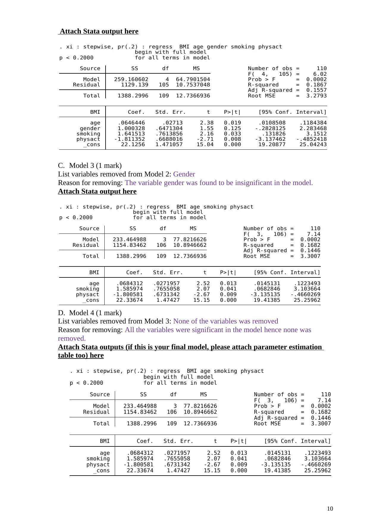
Attach Stata output here
_cons 22.1256 1.471057 15.04 0.000 19.20877 25.04243
physact -1.811352 .6688016 -2.71 0.008 -3.137462 -.4852418
smoking 1.641513 .7613856 2.16 0.033 .131826 3.1512
gender 1.000328 .6471304 1.55 0.125 -.2828125 2.283468
age .0646446 .02713 2.38 0.019 .0108508 .1184384
BMI Coef. Std. Err. t P>|t| [95% Conf. Interval]
Total 1388.2996 109 12.7366936 Root MSE = 3.2793
Adj R-squared = 0.1557
Residual 1129.139 105 10.7537048 R-squared = 0.1867
Model 259.160602 4 64.7901504 Prob > F = 0.0002
F( 4, 105) = 6.02
Source SS df MS Number of obs = 110
p < 0.2000 for all terms in model
begin with full model
. xi : stepwise, pr(.2) : regress BMI age gender smoking physact
C. Model 3 (1 mark)
List variables removed from Model 2: Gender
Reason for removing: The variable gender was found to be insignificant in the model.
Attach Stata output here
_cons 22.33674 1.47427 15.15 0.000 19.41385 25.25962
physact -1.800581 .6731342 -2.67 0.009 -3.135135 -.4660269
smoking 1.585974 .7655058 2.07 0.041 .0682846 3.103664
age .0684312 .0271957 2.52 0.013 .0145131 .1223493
BMI Coef. Std. Err. t P>|t| [95% Conf. Interval]
Total 1388.2996 109 12.7366936 Root MSE = 3.3007
Adj R-squared = 0.1446
Residual 1154.83462 106 10.8946662 R-squared = 0.1682
Model 233.464988 3 77.8216626 Prob > F = 0.0002
F( 3, 106) = 7.14
Source SS df MS Number of obs = 110
p < 0.2000 for all terms in model
begin with full model
. xi : stepwise, pr(.2) : regress BMI age smoking physact
D. Model 4 (1 mark)
List variables removed from Model 3: None of the variables was removed
Reason for removing: All the variables were significant in the model hence none was
removed.
Attach Stata outputs (if this is your final model, please attach parameter estimation
table too) here
_cons 22.33674 1.47427 15.15 0.000 19.41385 25.25962
physact -1.800581 .6731342 -2.67 0.009 -3.135135 -.4660269
smoking 1.585974 .7655058 2.07 0.041 .0682846 3.103664
age .0684312 .0271957 2.52 0.013 .0145131 .1223493
BMI Coef. Std. Err. t P>|t| [95% Conf. Interval]
Total 1388.2996 109 12.7366936 Root MSE = 3.3007
Adj R-squared = 0.1446
Residual 1154.83462 106 10.8946662 R-squared = 0.1682
Model 233.464988 3 77.8216626 Prob > F = 0.0002
F( 3, 106) = 7.14
Source SS df MS Number of obs = 110
p < 0.2000 for all terms in model
begin with full model
. xi : stepwise, pr(.2) : regress BMI age smoking physact
10
Paraphrase This Document
Need a fresh take? Get an instant paraphrase of this document with our AI Paraphraser
3 (4 marks)Assessment of assumptions for the final model obtained in Question 2 above (include
your interpretations and conclusions).
3.1 Assess and comment on the normality of the standardised residuals; (1 mark)
(No Stata output(s) are required for this question)
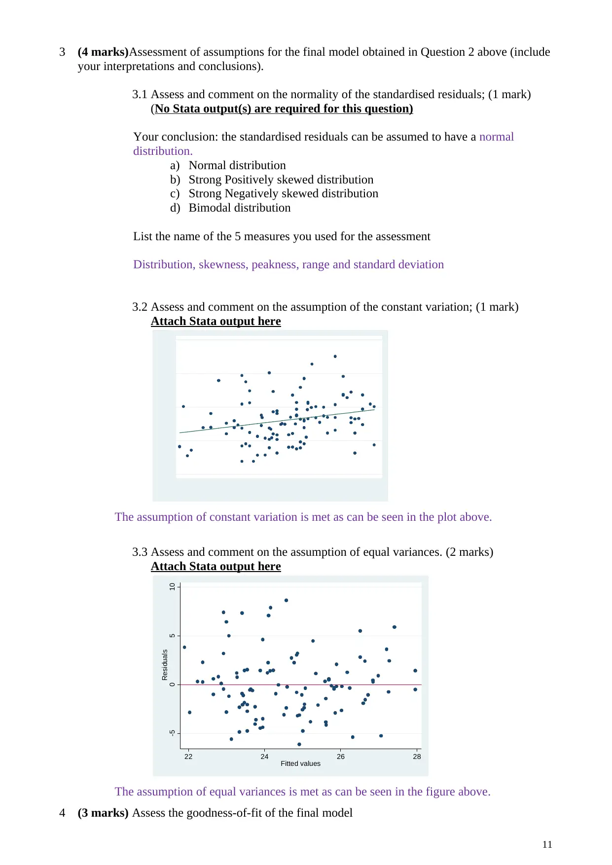
Your conclusion: the standardised residuals can be assumed to have a normal
distribution.
a) Normal distribution
b) Strong Positively skewed distribution
c) Strong Negatively skewed distribution
d) Bimodal distribution
List the name of the 5 measures you used for the assessment
Distribution, skewness, peakness, range and standard deviation
3.2 Assess and comment on the assumption of the constant variation; (1 mark)
Attach Stata output here
The assumption of constant variation is met as can be seen in the plot above.
3.3 Assess and comment on the assumption of equal variances. (2 marks)
Attach Stata output here
-5 0 5 10
Residuals
22 24 26 28
Fitted values
The assumption of equal variances is met as can be seen in the figure above.
4 (3 marks) Assess the goodness-of-fit of the final model
11
(No Stata output(s) are required for this question)
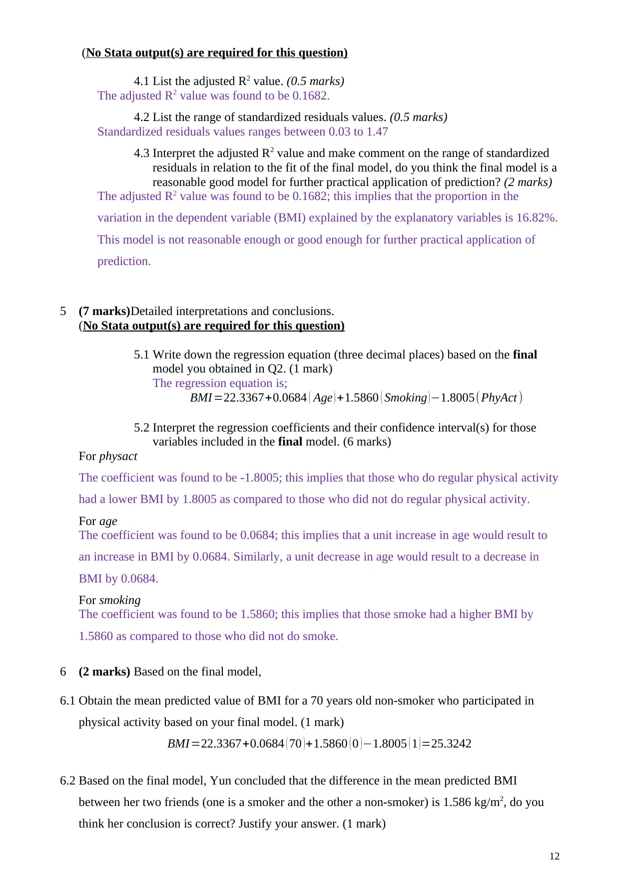
4.1 List the adjusted R2 value. (0.5 marks)
The adjusted R2 value was found to be 0.1682.
4.2 List the range of standardized residuals values. (0.5 marks)
Standardized residuals values ranges between 0.03 to 1.47
4.3 Interpret the adjusted R2 value and make comment on the range of standardized
residuals in relation to the fit of the final model, do you think the final model is a
reasonable good model for further practical application of prediction? (2 marks)
The adjusted R2 value was found to be 0.1682; this implies that the proportion in the
variation in the dependent variable (BMI) explained by the explanatory variables is 16.82%.
This model is not reasonable enough or good enough for further practical application of
prediction.
5 (7 marks)Detailed interpretations and conclusions.
(No Stata output(s) are required for this question)
5.1 Write down the regression equation (three decimal places) based on the final
model you obtained in Q2. (1 mark)
The regression equation is;
BMI =22.3367+0.0684 ( Age ) +1.5860 ( Smoking ) −1.8005(PhyAct )
5.2 Interpret the regression coefficients and their confidence interval(s) for those
variables included in the final model. (6 marks)
For physact
The coefficient was found to be -1.8005; this implies that those who do regular physical activity
had a lower BMI by 1.8005 as compared to those who did not do regular physical activity.
For age
The coefficient was found to be 0.0684; this implies that a unit increase in age would result to
an increase in BMI by 0.0684. Similarly, a unit decrease in age would result to a decrease in
BMI by 0.0684.
For smoking
The coefficient was found to be 1.5860; this implies that those smoke had a higher BMI by
1.5860 as compared to those who did not do smoke.
6 (2 marks) Based on the final model,
6.1 Obtain the mean predicted value of BMI for a 70 years old non-smoker who participated in
physical activity based on your final model. (1 mark)
BMI=22.3367+0.0684 ( 70 )+1.5860 ( 0 )−1.8005 ( 1 )=25.3242
6.2 Based on the final model, Yun concluded that the difference in the mean predicted BMI
between her two friends (one is a smoker and the other a non-smoker) is 1.586 kg/m2, do you
think her conclusion is correct? Justify your answer. (1 mark)
12
⊘ This is a preview!⊘
Do you want full access?
Subscribe today to unlock all pages.

Trusted by 1+ million students worldwide
1 out of 13
Related Documents
Your All-in-One AI-Powered Toolkit for Academic Success.
+13062052269
info@desklib.com
Available 24*7 on WhatsApp / Email
![[object Object]](/_next/static/media/star-bottom.7253800d.svg)
Unlock your academic potential
Copyright © 2020–2026 A2Z Services. All Rights Reserved. Developed and managed by ZUCOL.


