PUBH620 Biostatistics Assignment: Data Analysis and Interpretation
VerifiedAdded on 2023/01/19
|16
|2947
|51
Homework Assignment
AI Summary
This biostatistics assignment analyzes a dataset from a longitudinal survey of ACU student health and wellbeing. The assignment includes descriptive statistics, frequency tables, and independent samples t-tests to compare means across different demographic and status groups. The analysis co...
Running head: BIOSTATISTICS ASSIGNMENT 1
Biostatistics Assignment
By (Student name)
(Institutional Affiliation)
(Date of Submission)
Biostatistics Assignment
By (Student name)
(Institutional Affiliation)
(Date of Submission)
Paraphrase This Document
Need a fresh take? Get an instant paraphrase of this document with our AI Paraphraser
BIOSTATISTICS ASSIGNMENT 2
Question 1
a. Age summary statistics
Statistics
AGE
N Valid 38681
Missing 0
Mean 20.50
Std. Deviation 4.888
Minimum 16
Maximum 59
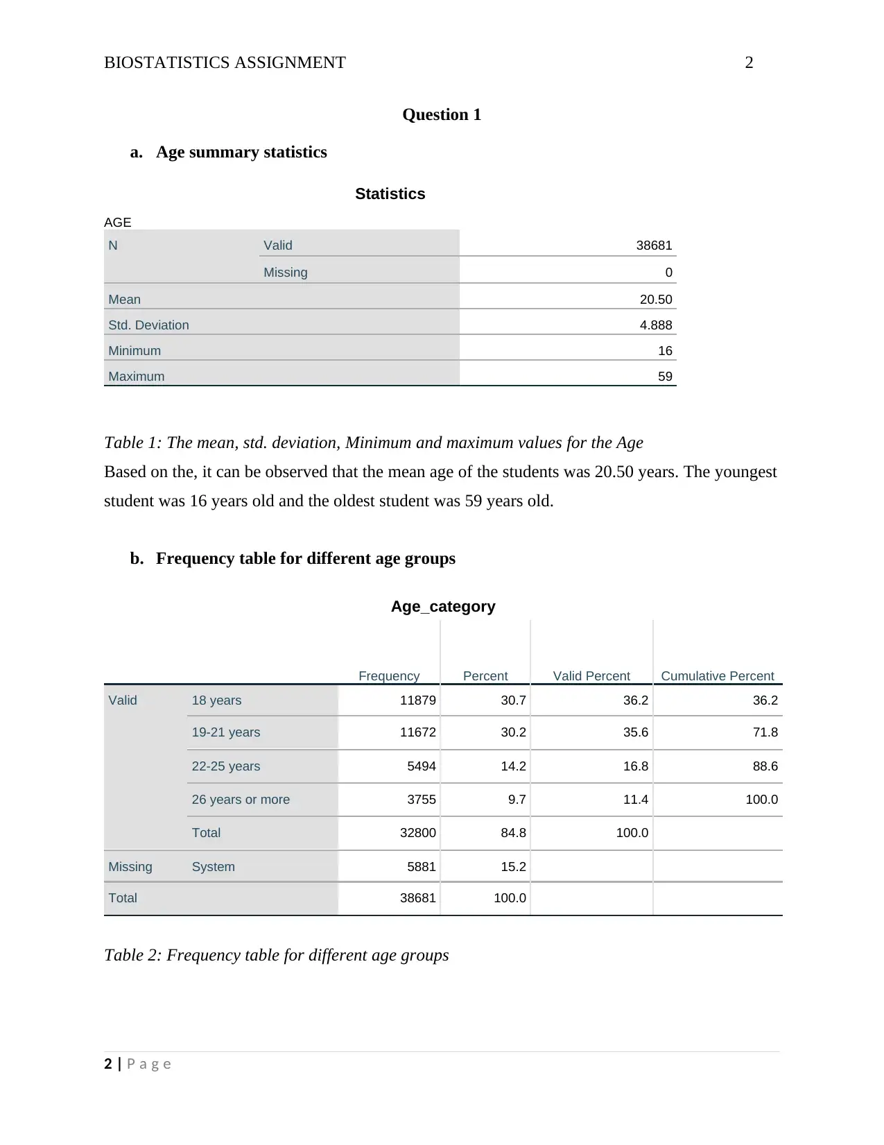
Table 1: The mean, std. deviation, Minimum and maximum values for the Age
Based on the, it can be observed that the mean age of the students was 20.50 years. The youngest
student was 16 years old and the oldest student was 59 years old.
b. Frequency table for different age groups
Age_category
Frequency Percent Valid Percent Cumulative Percent
Valid 18 years 11879 30.7 36.2 36.2
19-21 years 11672 30.2 35.6 71.8
22-25 years 5494 14.2 16.8 88.6
26 years or more 3755 9.7 11.4 100.0
Total 32800 84.8 100.0
Missing System 5881 15.2
Total 38681 100.0
Table 2: Frequency table for different age groups
2 | P a g e
BIOSTATISTICS ASSIGNMENT 3
The table 2 above distributed the student in terms of age groups. Students who are 18 years are
11879 (30.7%). Students who are 19-21 years are 11672 (30.2%). Those who are 22-25 years are
5494 (14.2%). Those who are 26 years and above were 3755 (9.7%).
Question 2
Frequency statistics cohort table
cohort
Frequency Percent Valid Percent
Cumulative
Percent
Valid 2005 3259 8.4 8.4 8.4
2006 3615 9.3 9.3 17.8
2007 3944 10.2 10.2 28.0
2008 4086 10.6 10.6 38.5
2009 5010 13.0 13.0 51.5
2010 5687 14.7 14.7 66.2
2011 6383 16.5 16.5 82.7
2012 6697 17.3 17.3 100.0
Total 38681 100.0 100.0
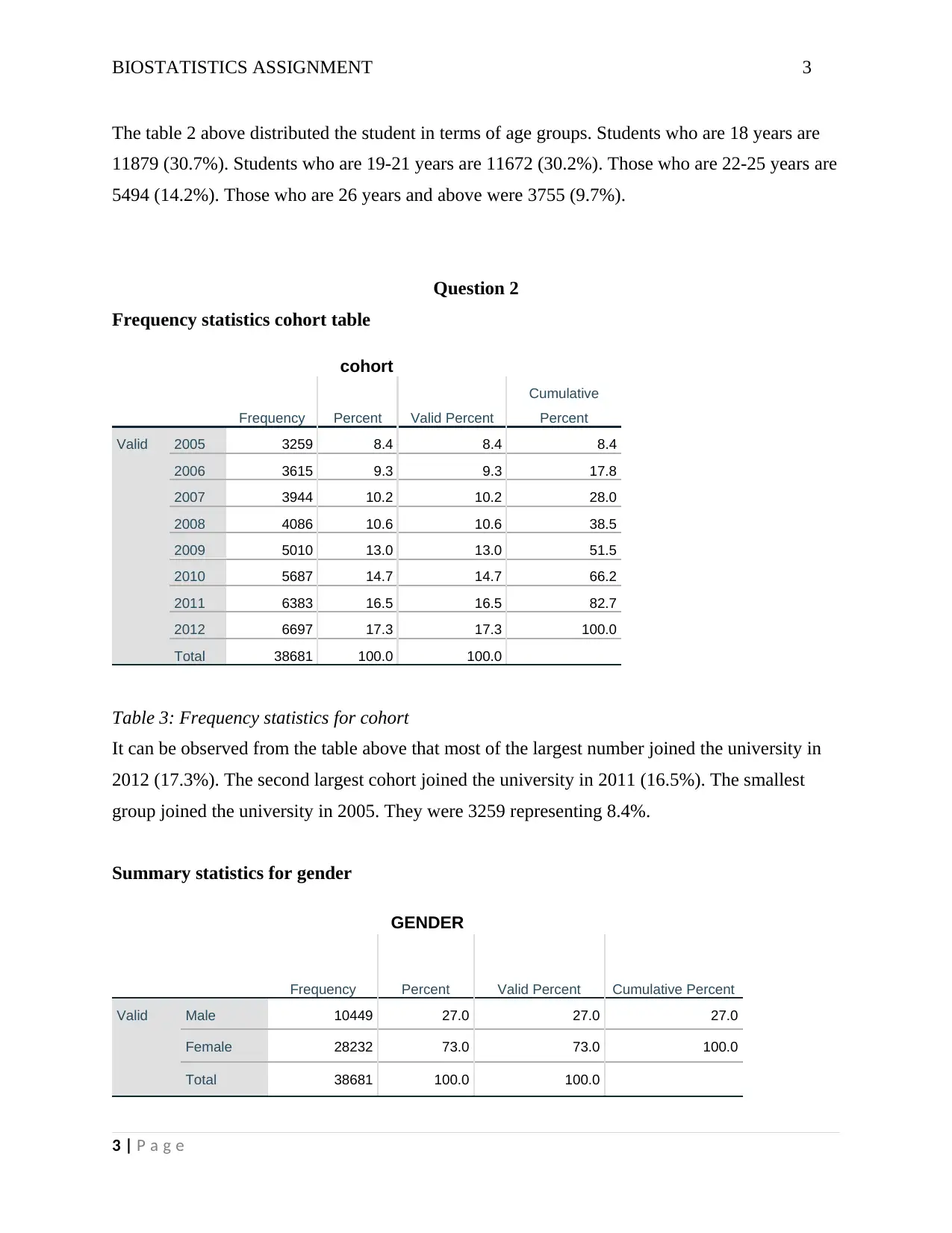
Table 3: Frequency statistics for cohort
It can be observed from the table above that most of the largest number joined the university in
2012 (17.3%). The second largest cohort joined the university in 2011 (16.5%). The smallest
group joined the university in 2005. They were 3259 representing 8.4%.
Summary statistics for gender
GENDER
Frequency Percent Valid Percent Cumulative Percent
Valid Male 10449 27.0 27.0 27.0
Female 28232 73.0 73.0 100.0
Total 38681 100.0 100.0
3 | P a g e
⊘ This is a preview!⊘
Do you want full access?
Subscribe today to unlock all pages.

Trusted by 1+ million students worldwide
BIOSTATISTICS ASSIGNMENT 4
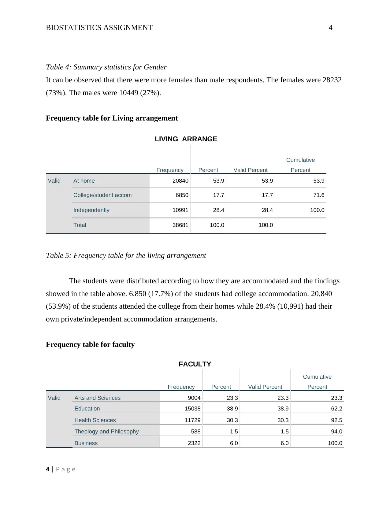
Table 4: Summary statistics for Gender
It can be observed that there were more females than male respondents. The females were 28232
(73%). The males were 10449 (27%).
Frequency table for Living arrangement
LIVING_ARRANGE
Frequency Percent Valid Percent
Cumulative
Percent
Valid At home 20840 53.9 53.9 53.9
College/student accom 6850 17.7 17.7 71.6
Independently 10991 28.4 28.4 100.0
Total 38681 100.0 100.0
Table 5: Frequency table for the living arrangement
The students were distributed according to how they are accommodated and the findings
showed in the table above. 6,850 (17.7%) of the students had college accommodation. 20,840
(53.9%) of the students attended the college from their homes while 28.4% (10,991) had their
own private/independent accommodation arrangements.
Frequency table for faculty
FACULTY
Frequency Percent Valid Percent
Cumulative
Percent
Valid Arts and Sciences 9004 23.3 23.3 23.3
Education 15038 38.9 38.9 62.2
Health Sciences 11729 30.3 30.3 92.5
Theology and Philosophy 588 1.5 1.5 94.0
Business 2322 6.0 6.0 100.0
4 | P a g e
Paraphrase This Document
Need a fresh take? Get an instant paraphrase of this document with our AI Paraphraser
BIOSTATISTICS ASSIGNMENT 5
Total 38681 100.0 100.0
Table 6: Frequency table for faculty
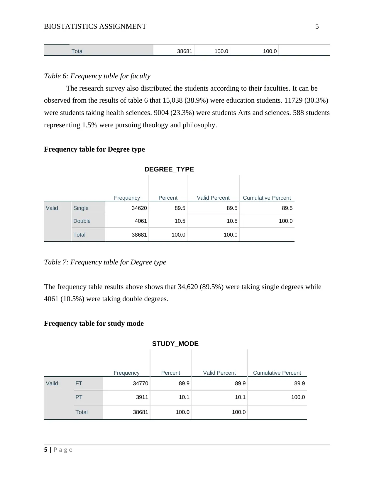
The research survey also distributed the students according to their faculties. It can be
observed from the results of table 6 that 15,038 (38.9%) were education students. 11729 (30.3%)
were students taking health sciences. 9004 (23.3%) were students Arts and sciences. 588 students
representing 1.5% were pursuing theology and philosophy.
Frequency table for Degree type
DEGREE_TYPE
Frequency Percent Valid Percent Cumulative Percent
Valid Single 34620 89.5 89.5 89.5
Double 4061 10.5 10.5 100.0
Total 38681 100.0 100.0
Table 7: Frequency table for Degree type
The frequency table results above shows that 34,620 (89.5%) were taking single degrees while
4061 (10.5%) were taking double degrees.
Frequency table for study mode
STUDY_MODE
Frequency Percent Valid Percent Cumulative Percent
Valid FT 34770 89.9 89.9 89.9
PT 3911 10.1 10.1 100.0
Total 38681 100.0 100.0
5 | P a g e
Total 38681 100.0 100.0
Table 6: Frequency table for faculty
The research survey also distributed the students according to their faculties. It can be
observed from the results of table 6 that 15,038 (38.9%) were education students. 11729 (30.3%)
were students taking health sciences. 9004 (23.3%) were students Arts and sciences. 588 students
representing 1.5% were pursuing theology and philosophy.
Frequency table for Degree type
DEGREE_TYPE
Frequency Percent Valid Percent Cumulative Percent
Valid Single 34620 89.5 89.5 89.5
Double 4061 10.5 10.5 100.0
Total 38681 100.0 100.0
Table 7: Frequency table for Degree type
The frequency table results above shows that 34,620 (89.5%) were taking single degrees while
4061 (10.5%) were taking double degrees.
Frequency table for study mode
STUDY_MODE
Frequency Percent Valid Percent Cumulative Percent
Valid FT 34770 89.9 89.9 89.9
PT 3911 10.1 10.1 100.0
Total 38681 100.0 100.0
5 | P a g e
BIOSTATISTICS ASSIGNMENT 6
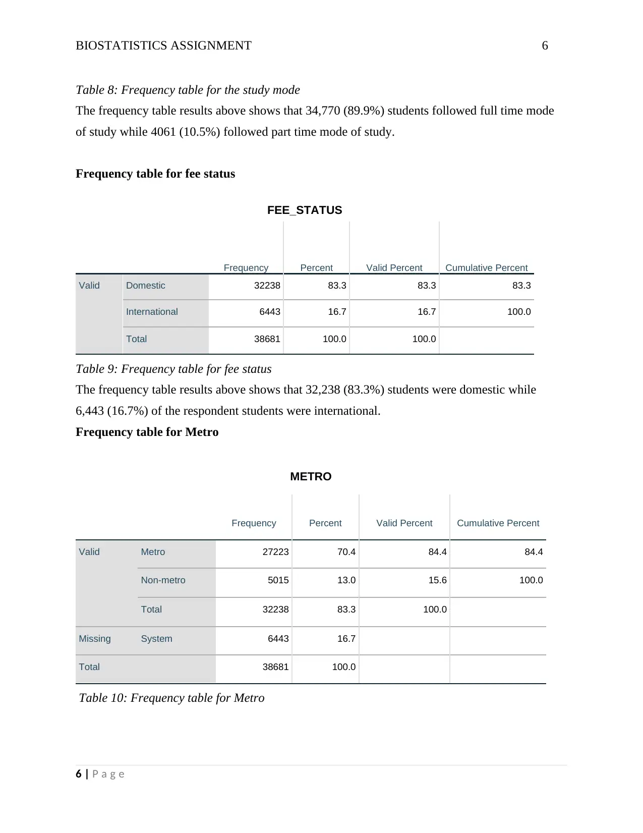
Table 8: Frequency table for the study mode
The frequency table results above shows that 34,770 (89.9%) students followed full time mode
of study while 4061 (10.5%) followed part time mode of study.
Frequency table for fee status
FEE_STATUS
Frequency Percent Valid Percent Cumulative Percent
Valid Domestic 32238 83.3 83.3 83.3
International 6443 16.7 16.7 100.0
Total 38681 100.0 100.0
Table 9: Frequency table for fee status
The frequency table results above shows that 32,238 (83.3%) students were domestic while
6,443 (16.7%) of the respondent students were international.
Frequency table for Metro
METRO
Frequency Percent Valid Percent Cumulative Percent
Valid Metro 27223 70.4 84.4 84.4
Non-metro 5015 13.0 15.6 100.0
Total 32238 83.3 100.0
Missing System 6443 16.7
Total 38681 100.0
Table 10: Frequency table for Metro
6 | P a g e
⊘ This is a preview!⊘
Do you want full access?
Subscribe today to unlock all pages.

Trusted by 1+ million students worldwide
BIOSTATISTICS ASSIGNMENT 7
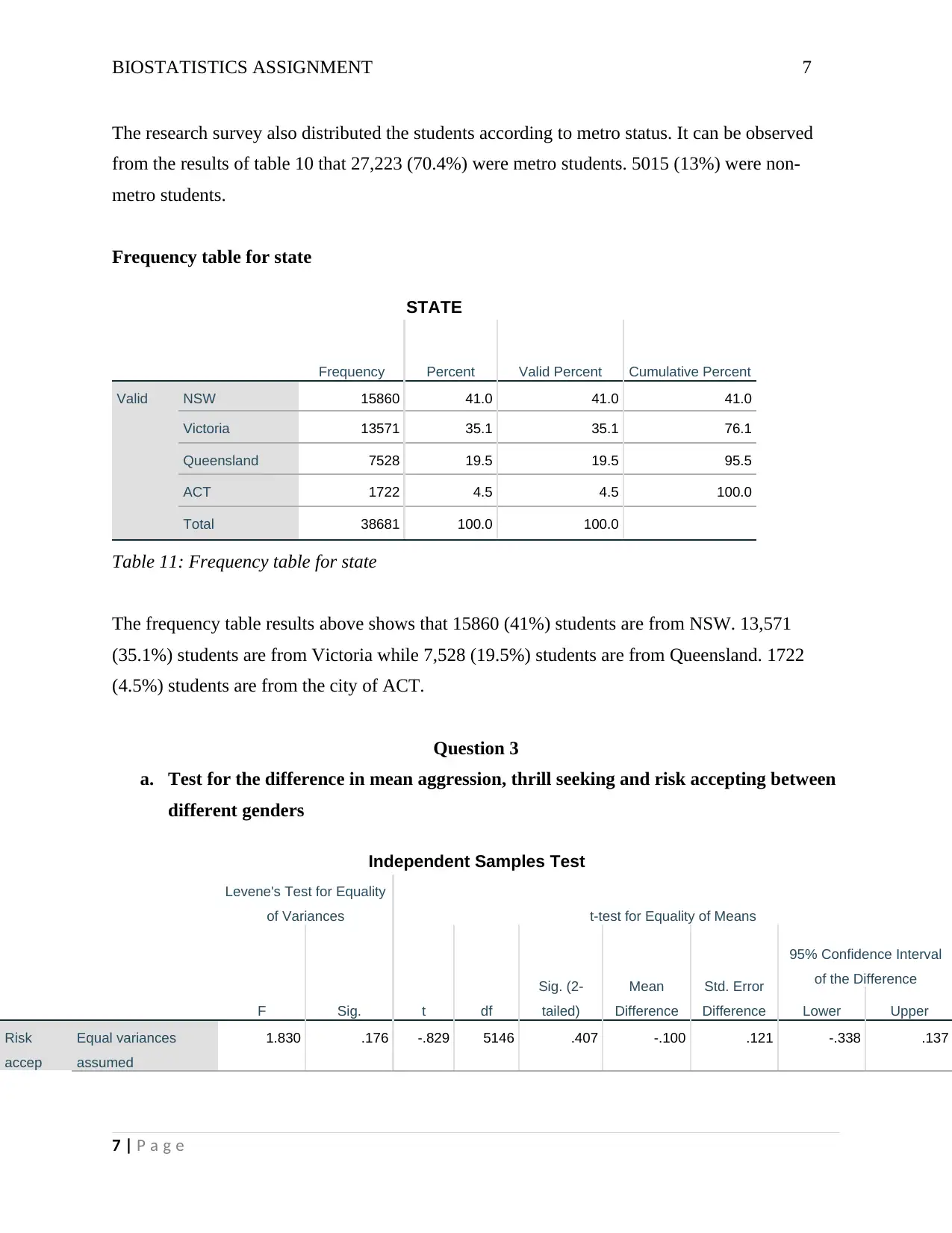
The research survey also distributed the students according to metro status. It can be observed
from the results of table 10 that 27,223 (70.4%) were metro students. 5015 (13%) were non-
metro students.
Frequency table for state
STATE
Frequency Percent Valid Percent Cumulative Percent
Valid NSW 15860 41.0 41.0 41.0
Victoria 13571 35.1 35.1 76.1
Queensland 7528 19.5 19.5 95.5
ACT 1722 4.5 4.5 100.0
Total 38681 100.0 100.0
Table 11: Frequency table for state
The frequency table results above shows that 15860 (41%) students are from NSW. 13,571
(35.1%) students are from Victoria while 7,528 (19.5%) students are from Queensland. 1722
(4.5%) students are from the city of ACT.
Question 3
a. Test for the difference in mean aggression, thrill seeking and risk accepting between
different genders
Independent Samples Test
Levene's Test for Equality
of Variances t-test for Equality of Means
F Sig. t df
Sig. (2-
tailed)
Mean
Difference
Std. Error
Difference
95% Confidence Interval
of the Difference
Lower Upper
Risk
accep
Equal variances
assumed
1.830 .176 -.829 5146 .407 -.100 .121 -.338 .137
7 | P a g e
Paraphrase This Document
Need a fresh take? Get an instant paraphrase of this document with our AI Paraphraser
BIOSTATISTICS ASSIGNMENT 8
Equal variances not
assumed
-.829 5145.97
8
.407 -.100 .121 -.338 .137
thrill Equal variances
assumed
40881.922 .000 -65.305 5146 .000 -.622 .010 -.641 -.603
Equal variances not
assumed
-64.849 2555.00
0
.000 -.622 .010 -.641 -.603
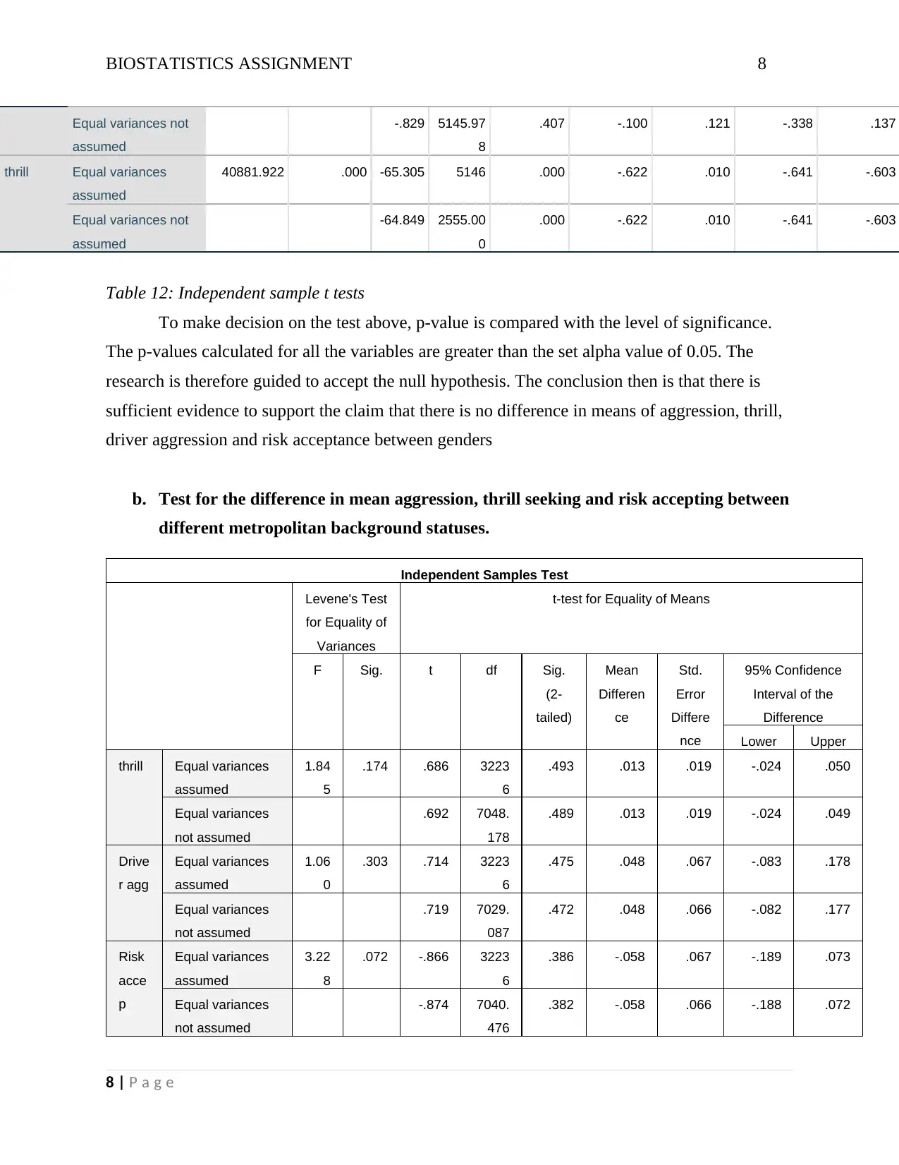
Table 12: Independent sample t tests
To make decision on the test above, p-value is compared with the level of significance.
The p-values calculated for all the variables are greater than the set alpha value of 0.05. The
research is therefore guided to accept the null hypothesis. The conclusion then is that there is
sufficient evidence to support the claim that there is no difference in means of aggression, thrill,
driver aggression and risk acceptance between genders
b. Test for the difference in mean aggression, thrill seeking and risk accepting between
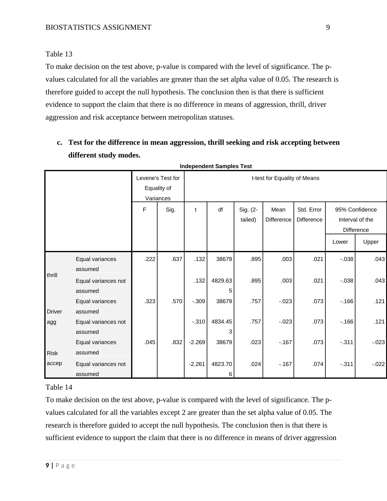
different metropolitan background statuses.
Independent Samples Test
Levene's Test
for Equality of
Variances
t-test for Equality of Means
F Sig. t df Sig.
(2-
tailed)
Mean
Differen
ce
Std.
Error
Differe
nce
95% Confidence
Interval of the
Difference
Lower Upper
thrill Equal variances
assumed
1.84
5
.174 .686 3223
6
.493 .013 .019 -.024 .050
Equal variances
not assumed
.692 7048.
178
.489 .013 .019 -.024 .049
Drive
r agg
Equal variances
assumed
1.06
0
.303 .714 3223
6
.475 .048 .067 -.083 .178
Equal variances
not assumed
.719 7029.
087
.472 .048 .066 -.082 .177
Risk
acce
p
Equal variances
assumed
3.22
8
.072 -.866 3223
6
.386 -.058 .067 -.189 .073
Equal variances
not assumed
-.874 7040.
476
.382 -.058 .066 -.188 .072
8 | P a g e
Equal variances not
assumed
-.829 5145.97
8
.407 -.100 .121 -.338 .137
thrill Equal variances
assumed
40881.922 .000 -65.305 5146 .000 -.622 .010 -.641 -.603
Equal variances not
assumed
-64.849 2555.00
0
.000 -.622 .010 -.641 -.603
Table 12: Independent sample t tests
To make decision on the test above, p-value is compared with the level of significance.
The p-values calculated for all the variables are greater than the set alpha value of 0.05. The
research is therefore guided to accept the null hypothesis. The conclusion then is that there is
sufficient evidence to support the claim that there is no difference in means of aggression, thrill,
driver aggression and risk acceptance between genders
b. Test for the difference in mean aggression, thrill seeking and risk accepting between
different metropolitan background statuses.
Independent Samples Test
Levene's Test
for Equality of
Variances
t-test for Equality of Means
F Sig. t df Sig.
(2-
tailed)
Mean
Differen
ce
Std.
Error
Differe
nce
95% Confidence
Interval of the
Difference
Lower Upper
thrill Equal variances
assumed
1.84
5
.174 .686 3223
6
.493 .013 .019 -.024 .050
Equal variances
not assumed
.692 7048.
178
.489 .013 .019 -.024 .049
Drive
r agg
Equal variances
assumed
1.06
0
.303 .714 3223
6
.475 .048 .067 -.083 .178
Equal variances
not assumed
.719 7029.
087
.472 .048 .066 -.082 .177
Risk
acce
p
Equal variances
assumed
3.22
8
.072 -.866 3223
6
.386 -.058 .067 -.189 .073
Equal variances
not assumed
-.874 7040.
476
.382 -.058 .066 -.188 .072
8 | P a g e
BIOSTATISTICS ASSIGNMENT 9
Table 13
To make decision on the test above, p-value is compared with the level of significance. The p-
values calculated for all the variables are greater than the set alpha value of 0.05. The research is
therefore guided to accept the null hypothesis. The conclusion then is that there is sufficient
evidence to support the claim that there is no difference in means of aggression, thrill, driver
aggression and risk acceptance between metropolitan statuses.
c. Test for the difference in mean aggression, thrill seeking and risk accepting between
different study modes.
Independent Samples Test
Levene's Test for
Equality of
Variances
t-test for Equality of Means
F Sig. t df Sig. (2-
tailed)
Mean
Difference
Std. Error
Difference
95% Confidence
Interval of the
Difference
Lower Upper
thrill
Equal variances
assumed
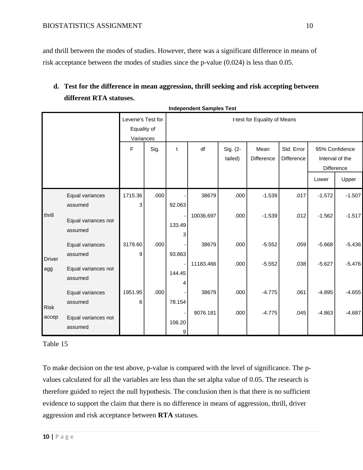
.222 .637 .132 38679 .895 .003 .021 -.038 .043
Equal variances not
assumed
.132 4829.63
5
.895 .003 .021 -.038 .043
Driver
agg
Equal variances
assumed
.323 .570 -.309 38679 .757 -.023 .073 -.166 .121
Equal variances not
assumed
-.310 4834.45
3
.757 -.023 .073 -.166 .121
Risk
accep
Equal variances
assumed
.045 .832 -2.269 38679 .023 -.167 .073 -.311 -.023
Equal variances not
assumed
-2.261 4823.70
6
.024 -.167 .074 -.311 -.022
Table 14
To make decision on the test above, p-value is compared with the level of significance. The p-
values calculated for all the variables except 2 are greater than the set alpha value of 0.05. The
research is therefore guided to accept the null hypothesis. The conclusion then is that there is
sufficient evidence to support the claim that there is no difference in means of driver aggression
9 | P a g e
⊘ This is a preview!⊘
Do you want full access?
Subscribe today to unlock all pages.

Trusted by 1+ million students worldwide
BIOSTATISTICS ASSIGNMENT 10
and thrill between the modes of studies. However, there was a significant difference in means of
risk acceptance between the modes of studies since the p-value (0.024) is less than 0.05.
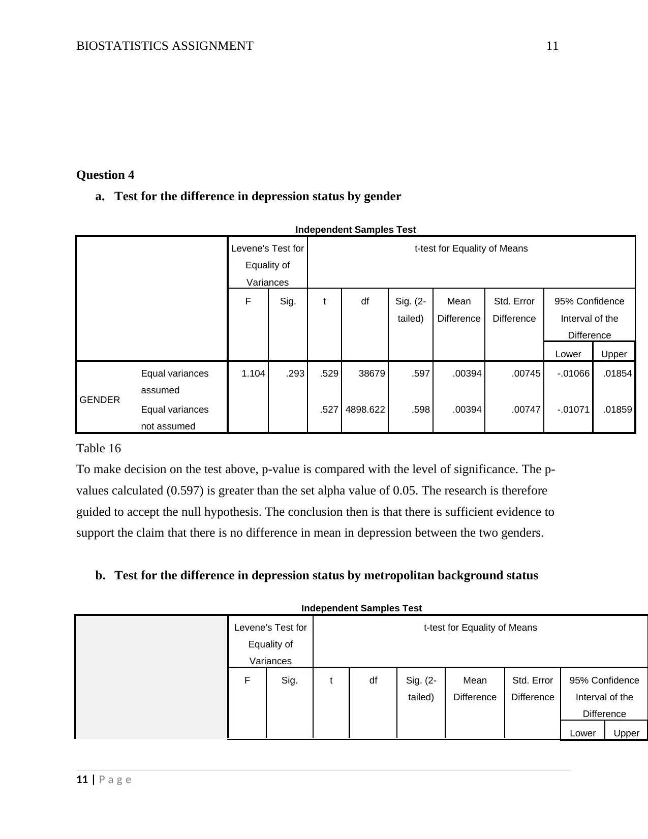
d. Test for the difference in mean aggression, thrill seeking and risk accepting between
different RTA statuses.
Independent Samples Test
Levene's Test for
Equality of
Variances
t-test for Equality of Means
F Sig. t df Sig. (2-
tailed)
Mean
Difference
Std. Error
Difference
95% Confidence
Interval of the
Difference
Lower Upper
thrill
Equal variances
assumed
1715.36
3
.000 -
92.063
38679 .000 -1.539 .017 -1.572 -1.507
Equal variances not
assumed
-
133.49
3
10036.697 .000 -1.539 .012 -1.562 -1.517
Driver
agg
Equal variances
assumed
3179.60
9
.000 -
93.863
38679 .000 -5.552 .059 -5.668 -5.436
Equal variances not
assumed
-
144.45
4
11183.466 .000 -5.552 .038 -5.627 -5.476
Risk
accep
Equal variances
assumed
1951.95
6
.000 -
78.154
38679 .000 -4.775 .061 -4.895 -4.655
Equal variances not
assumed
-
106.20
9
9076.181 .000 -4.775 .045 -4.863 -4.687
Table 15
To make decision on the test above, p-value is compared with the level of significance. The p-
values calculated for all the variables are less than the set alpha value of 0.05. The research is
therefore guided to reject the null hypothesis. The conclusion then is that there is no sufficient
evidence to support the claim that there is no difference in means of aggression, thrill, driver
aggression and risk acceptance between RTA statuses.
10 | P a g e
Paraphrase This Document
Need a fresh take? Get an instant paraphrase of this document with our AI Paraphraser
BIOSTATISTICS ASSIGNMENT 11
Question 4
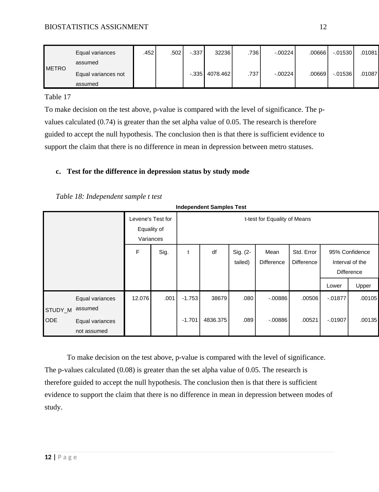
a. Test for the difference in depression status by gender
Independent Samples Test
Levene's Test for
Equality of
Variances
t-test for Equality of Means
F Sig. t df Sig. (2-
tailed)
Mean
Difference
Std. Error
Difference
95% Confidence
Interval of the
Difference
Lower Upper
GENDER
Equal variances
assumed
1.104 .293 .529 38679 .597 .00394 .00745 -.01066 .01854
Equal variances
not assumed
.527 4898.622 .598 .00394 .00747 -.01071 .01859
Table 16
To make decision on the test above, p-value is compared with the level of significance. The p-
values calculated (0.597) is greater than the set alpha value of 0.05. The research is therefore
guided to accept the null hypothesis. The conclusion then is that there is sufficient evidence to
support the claim that there is no difference in mean in depression between the two genders.
b. Test for the difference in depression status by metropolitan background status
Independent Samples Test
Levene's Test for
Equality of
Variances
t-test for Equality of Means
F Sig. t df Sig. (2-
tailed)
Mean
Difference
Std. Error
Difference
95% Confidence
Interval of the
Difference
Lower Upper
11 | P a g e
BIOSTATISTICS ASSIGNMENT 12
METRO
Equal variances
assumed
.452 .502 -.337 32236 .736 -.00224 .00666 -.01530 .01081
Equal variances not
assumed
-.335 4078.462 .737 -.00224 .00669 -.01536 .01087
Table 17
To make decision on the test above, p-value is compared with the level of significance. The p-
values calculated (0.74) is greater than the set alpha value of 0.05. The research is therefore
guided to accept the null hypothesis. The conclusion then is that there is sufficient evidence to
support the claim that there is no difference in mean in depression between metro statuses.
c. Test for the difference in depression status by study mode
Table 18: Independent sample t test
Independent Samples Test
Levene's Test for
Equality of
Variances
t-test for Equality of Means
F Sig. t df Sig. (2-
tailed)
Mean
Difference
Std. Error
Difference
95% Confidence
Interval of the
Difference
Lower Upper
STUDY_M
ODE
Equal variances
assumed
12.076 .001 -1.753 38679 .080 -.00886 .00506 -.01877 .00105
Equal variances
not assumed
-1.701 4836.375 .089 -.00886 .00521 -.01907 .00135
To make decision on the test above, p-value is compared with the level of significance.
The p-values calculated (0.08) is greater than the set alpha value of 0.05. The research is
therefore guided to accept the null hypothesis. The conclusion then is that there is sufficient
evidence to support the claim that there is no difference in mean in depression between modes of
study.
12 | P a g e
⊘ This is a preview!⊘
Do you want full access?
Subscribe today to unlock all pages.

Trusted by 1+ million students worldwide
BIOSTATISTICS ASSIGNMENT 13
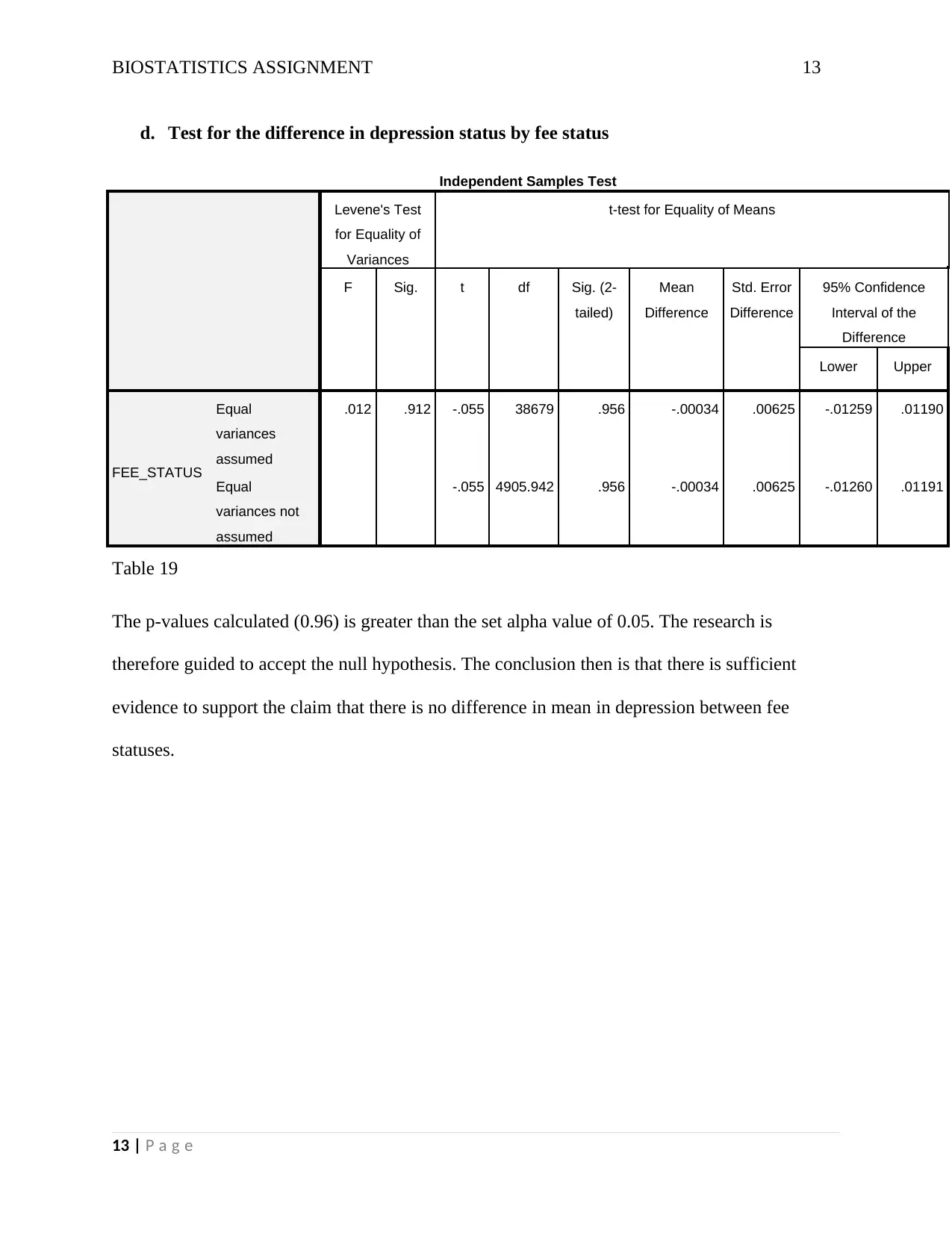
d. Test for the difference in depression status by fee status
Independent Samples Test
Levene's Test
for Equality of
Variances
t-test for Equality of Means
F Sig. t df Sig. (2-
tailed)
Mean
Difference
Std. Error
Difference
95% Confidence
Interval of the
Difference
Lower Upper
FEE_STATUS
Equal
variances
assumed
.012 .912 -.055 38679 .956 -.00034 .00625 -.01259 .01190
Equal
variances not
assumed
-.055 4905.942 .956 -.00034 .00625 -.01260 .01191
Table 19
The p-values calculated (0.96) is greater than the set alpha value of 0.05. The research is
therefore guided to accept the null hypothesis. The conclusion then is that there is sufficient
evidence to support the claim that there is no difference in mean in depression between fee
statuses.
13 | P a g e
Paraphrase This Document
Need a fresh take? Get an instant paraphrase of this document with our AI Paraphraser
BIOSTATISTICS ASSIGNMENT 14
Question 5
Binary logistics regression
a. Table of results
Variables in the Equation
B S.E. Wald df Sig. Exp(B) 95% C.I.for EXP(B)
Lower Upper
Step 1a
AGE -.052 .006 79.986 1 .000 .949 .938 .960
GENDER -.616 .052 139.183 1 .000 .540 .488 .599
LIVING_ARRANGE .036 .031 1.370 1 .242 1.036 .976 1.101
FEE_STATUS .532 .066 65.224 1 .000 1.702 1.496 1.937
driver_agg .621 .024 663.539 1 .000 1.861 1.775 1.951
thrill .548 .079 47.880 1 .000 1.729 1.481 2.020
risk_accep .611 .010 3986.925 1 .000 1.842 1.807 1.877
dist_driving -.060 .049 1.509 1 .219 .942 .857 1.036
Constant -16.626 .346 2313.704 1 .000 .000
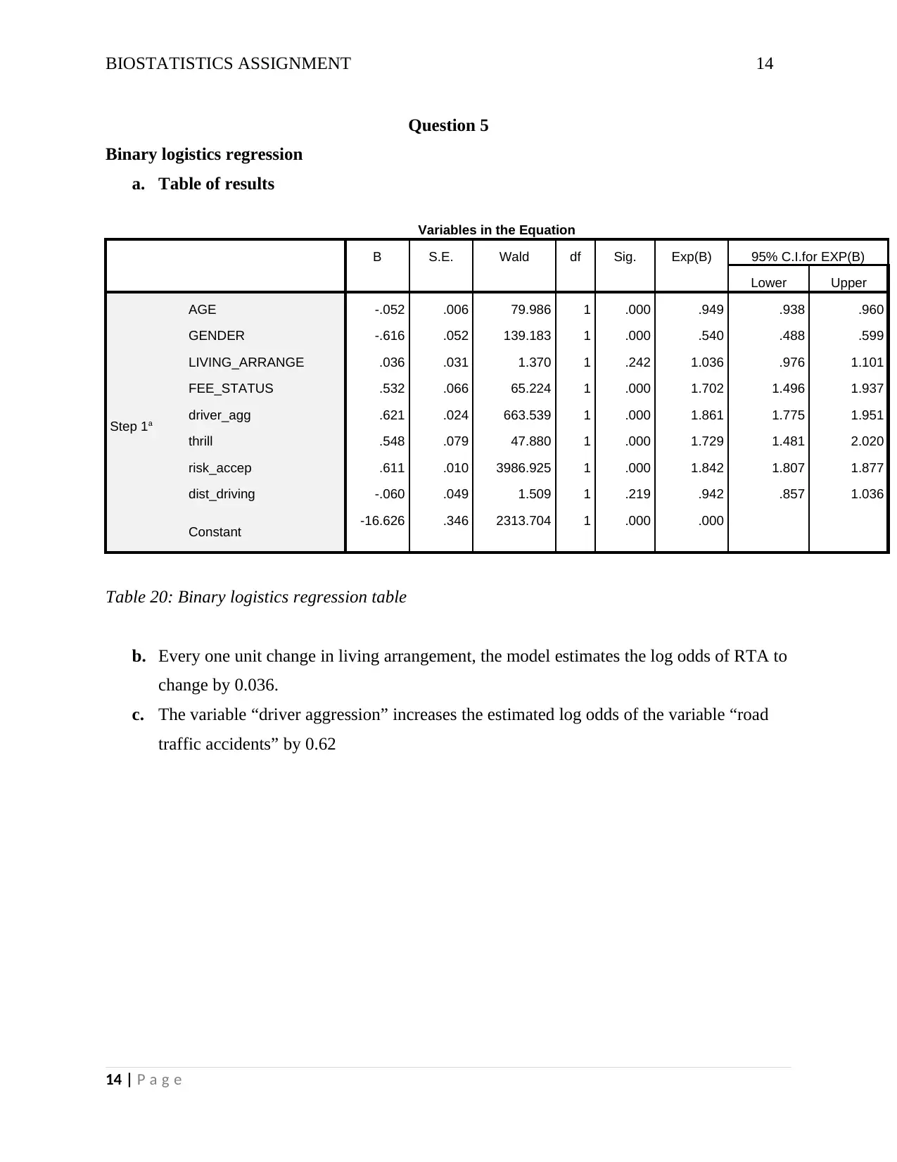
Table 20: Binary logistics regression table
b. Every one unit change in living arrangement, the model estimates the log odds of RTA to
change by 0.036.
c. The variable “driver aggression” increases the estimated log odds of the variable “road
traffic accidents” by 0.62
14 | P a g e
BIOSTATISTICS ASSIGNMENT 15
Question 6
a. Table of results
Variables in the Equation
B S.E. Wald df Sig. Exp(B) 95% C.I.for EXP(B)
Lower Upper
Step 1a
AGE -.035 .004 63.931 1 .000 .965 .957 .974
GENDER -.373 .039 92.415 1 .000 .688 .638 .743
LIVING_ARRANGE .063 .022 8.458 1 .004 1.065 1.021 1.110
depression 2.707 .056 2317.572 1 .000 14.978 13.416 16.723
owob_par 1.956 .170 131.591 1 .000 7.068 5.061 9.872
edu_par -2.654 .068 1514.337 1 .000 .070 .062 .080
BL_owob -.032 .037 .777 1 .378 .968 .901 1.040
Constant -2.268 .195 135.973 1 .000 .103
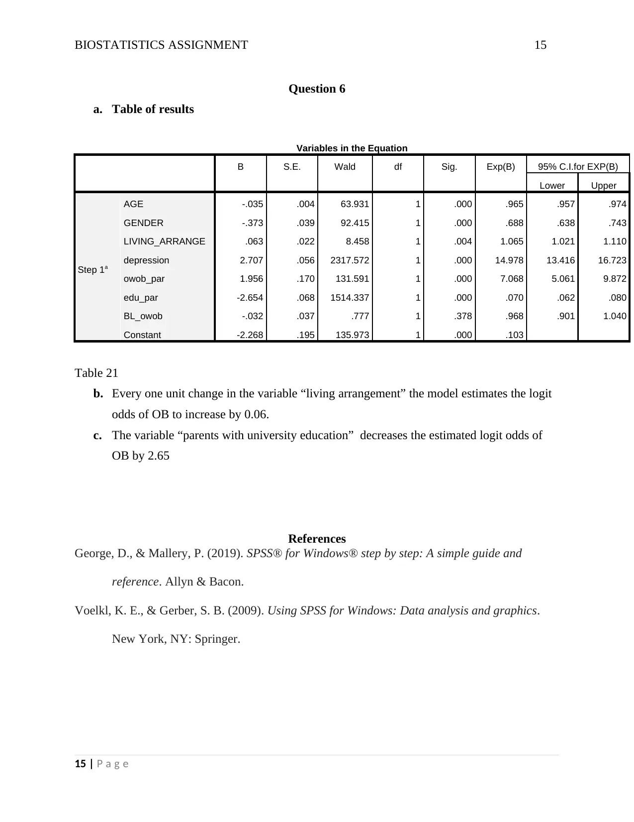
Table 21
b. Every one unit change in the variable “living arrangement” the model estimates the logit
odds of OB to increase by 0.06.
c. The variable “parents with university education” decreases the estimated logit odds of
OB by 2.65
References
George, D., & Mallery, P. (2019). SPSS® for Windows® step by step: A simple guide and
reference. Allyn & Bacon.
Voelkl, K. E., & Gerber, S. B. (2009). Using SPSS for Windows: Data analysis and graphics.
New York, NY: Springer.
15 | P a g e
⊘ This is a preview!⊘
Do you want full access?
Subscribe today to unlock all pages.

Trusted by 1+ million students worldwide

BIOSTATISTICS ASSIGNMENT 16
16 | P a g e
16 | P a g e
1 out of 16
Related Documents
Your All-in-One AI-Powered Toolkit for Academic Success.
+13062052269
info@desklib.com
Available 24*7 on WhatsApp / Email
![[object Object]](/_next/static/media/star-bottom.7253800d.svg)
Unlock your academic potential
© 2024 | Zucol Services PVT LTD | All rights reserved.


