Biostatistics for Public Health (TM5516) - Assignment 1

This document is a solved assignment on Biostatistics for Public Health (TM5516) - Assignment 1. It covers topics like cumulative distribution, conditional probability, probability calculations, null and alternate hypotheses, significance level, test statistic, confidence interval, frequency distribution, and summary statistics.

1
Biostatistics for Public Health (TM5516)
ASSIGNMENT 1

2
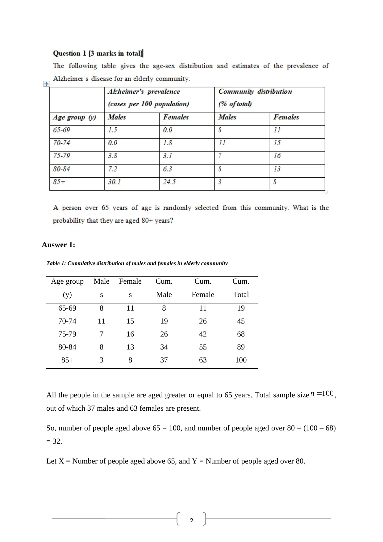
Answer 1:
Table 1: Cumulative distribution of males and females in elderly community
Age group
(y)
Male
s
Female
s
Cum.
Male
Cum.
Female
Cum.
Total
65-69 8 11 8 11 19
70-74 11 15 19 26 45
75-79 7 16 26 42 68
80-84 8 13 34 55 89
85+ 3 8 37 63 100
All the people in the sample are aged greater or equal to 65 years. Total sample size ,
out of which 37 males and 63 females are present.
So, number of people aged above 65 = 100, and number of people aged over 80 = (100 – 68)
= 32.
Let X = Number of people aged above 65, and Y = Number of people aged over 80.

3
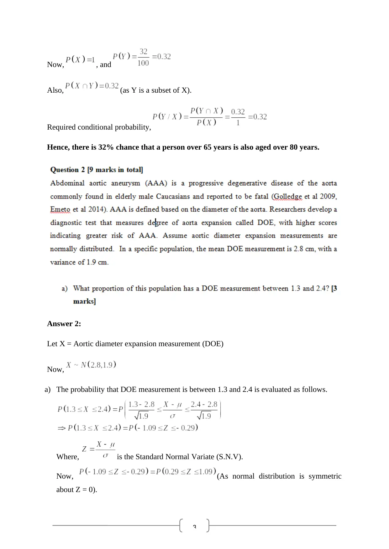
Now, , and
Also, (as Y is a subset of X).
Required conditional probability,
Hence, there is 32% chance that a person over 65 years is also aged over 80 years.
Answer 2:
Let X = Aortic diameter expansion measurement (DOE)
Now,
a) The probability that DOE measurement is between 1.3 and 2.4 is evaluated as follows.
Where, is the Standard Normal Variate (S.N.V).
Now, (As normal distribution is symmetric
about Z = 0).

4
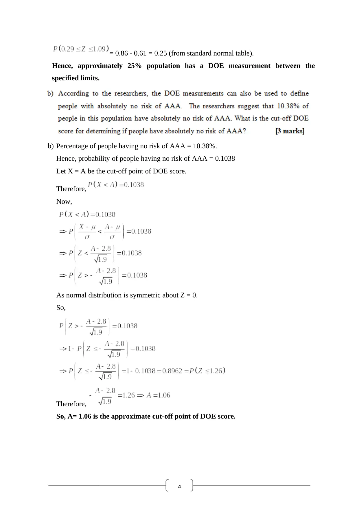
= 0.86 - 0.61 = 0.25 (from standard normal table).
Hence, approximately 25% population has a DOE measurement between the
specified limits.
b) Percentage of people having no risk of AAA = 10.38%.
Hence, probability of people having no risk of AAA = 0.1038
Let X = A be the cut-off point of DOE score.
Therefore,
Now,
As normal distribution is symmetric about Z = 0.
So,
Therefore,
So, A= 1.06 is the approximate cut-off point of DOE score.

5
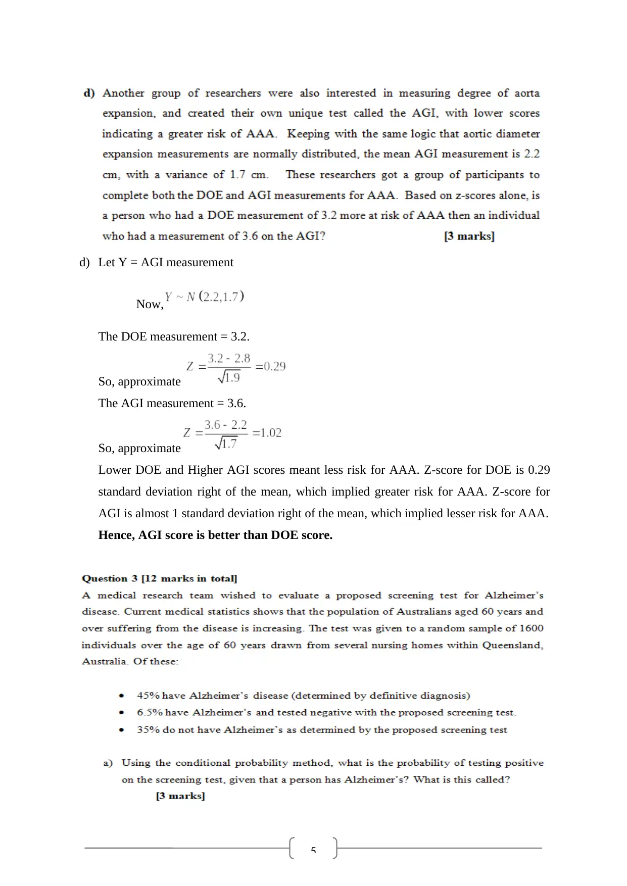
d) Let Y = AGI measurement
Now,
The DOE measurement = 3.2.
So, approximate
The AGI measurement = 3.6.
So, approximate
Lower DOE and Higher AGI scores meant less risk for AAA. Z-score for DOE is 0.29
standard deviation right of the mean, which implied greater risk for AAA. Z-score for
AGI is almost 1 standard deviation right of the mean, which implied lesser risk for AAA.
Hence, AGI score is better than DOE score.

6
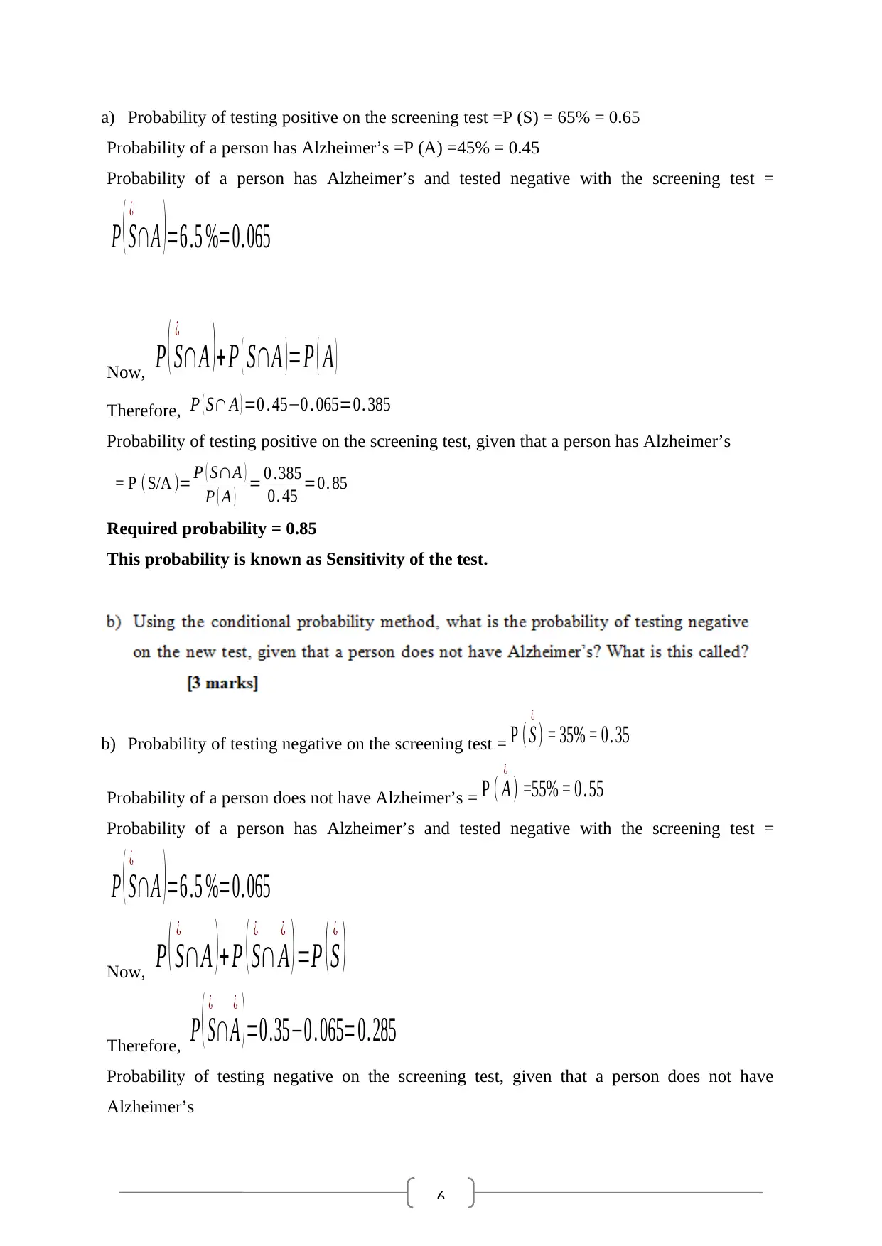
a) Probability of testing positive on the screening test =P (S) = 65% = 0.65
Probability of a person has Alzheimer’s =P (A) =45% = 0.45
Probability of a person has Alzheimer’s and tested negative with the screening test =
P ( S
¿
∩A ) =6 .5 %=0. 065
Now, P ( S
¿
∩A ) + P ( S∩A ) =P ( A )
Therefore, P ( S∩ A ) =0 . 45−0 . 065=0. 385
Probability of testing positive on the screening test, given that a person has Alzheimer’s
= P (S/A )= P ( S∩A )
P ( A ) = 0 .385
0. 45 =0. 85
Required probability = 0.85
This probability is known as Sensitivity of the test.
b) Probability of testing negative on the screening test = P ( S
¿
) = 35% = 0 . 35
Probability of a person does not have Alzheimer’s = P ( A
¿
) =55% = 0 . 55
Probability of a person has Alzheimer’s and tested negative with the screening test =
P ( S
¿
∩A ) =6 .5 %=0. 065
Now, P ( S
¿
∩A ) + P ( S
¿
∩ A
¿
) =P ( S
¿
)
Therefore, P ( S
¿
∩A
¿
) =0 .35−0 . 065=0. 285
Probability of testing negative on the screening test, given that a person does not have
Alzheimer’s

7
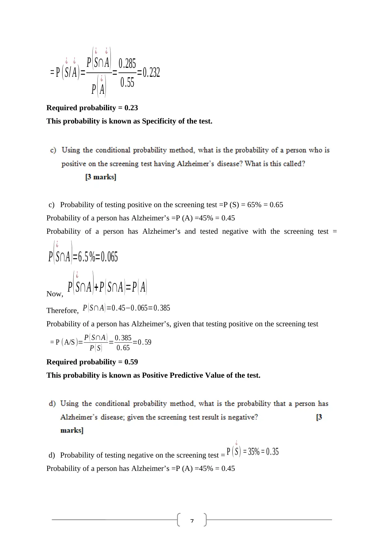
= P ( S
¿
/ A
¿
)= P ( S
¿
∩ A
¿
)
P ( A
¿
) = 0 .285
0 .55 =0. 232
Required probability = 0.23
This probability is known as Specificity of the test.
c) Probability of testing positive on the screening test =P (S) = 65% = 0.65
Probability of a person has Alzheimer’s =P (A) =45% = 0.45
Probability of a person has Alzheimer’s and tested negative with the screening test =
P ( S
¿
∩A ) =6 .5 %=0. 065
Now, P ( S
¿
∩A ) + P ( S∩A ) =P ( A )
Therefore, P ( S∩ A ) =0 . 45−0 . 065=0. 385
Probability of a person has Alzheimer’s, given that testing positive on the screening test
= P (A/S )= P ( S∩A )
P ( S ) = 0. 385
0. 65 =0 . 59
Required probability = 0.59
This probability is known as Positive Predictive Value of the test.
d) Probability of testing negative on the screening test = P ( S
¿
) = 35% = 0 . 35
Probability of a person has Alzheimer’s =P (A) =45% = 0.45

8
Probability of a person has Alzheimer’s and tested negative with the screening test =
P ( S
¿
∩A ) =6 .5 %=0. 065
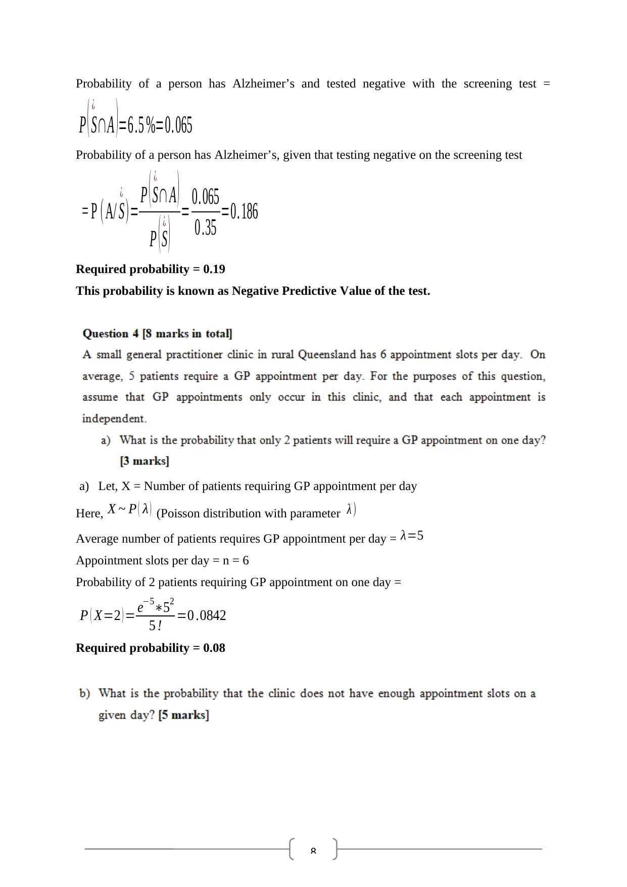
Probability of a person has Alzheimer’s, given that testing negative on the screening test
= P (A/ S
¿
)= P ( S
¿
∩ A )
P ( S
¿
) = 0. 065
0 .35 =0. 186
Required probability = 0.19
This probability is known as Negative Predictive Value of the test.
a) Let, X = Number of patients requiring GP appointment per day
Here, X ~ P ( λ ) (Poisson distribution with parameter λ )
Average number of patients requires GP appointment per day = λ=5
Appointment slots per day = n = 6
Probability of 2 patients requiring GP appointment on one day =
P ( X=2 ) = e−5∗52
5 ! =0 .0842
Required probability = 0.08

9
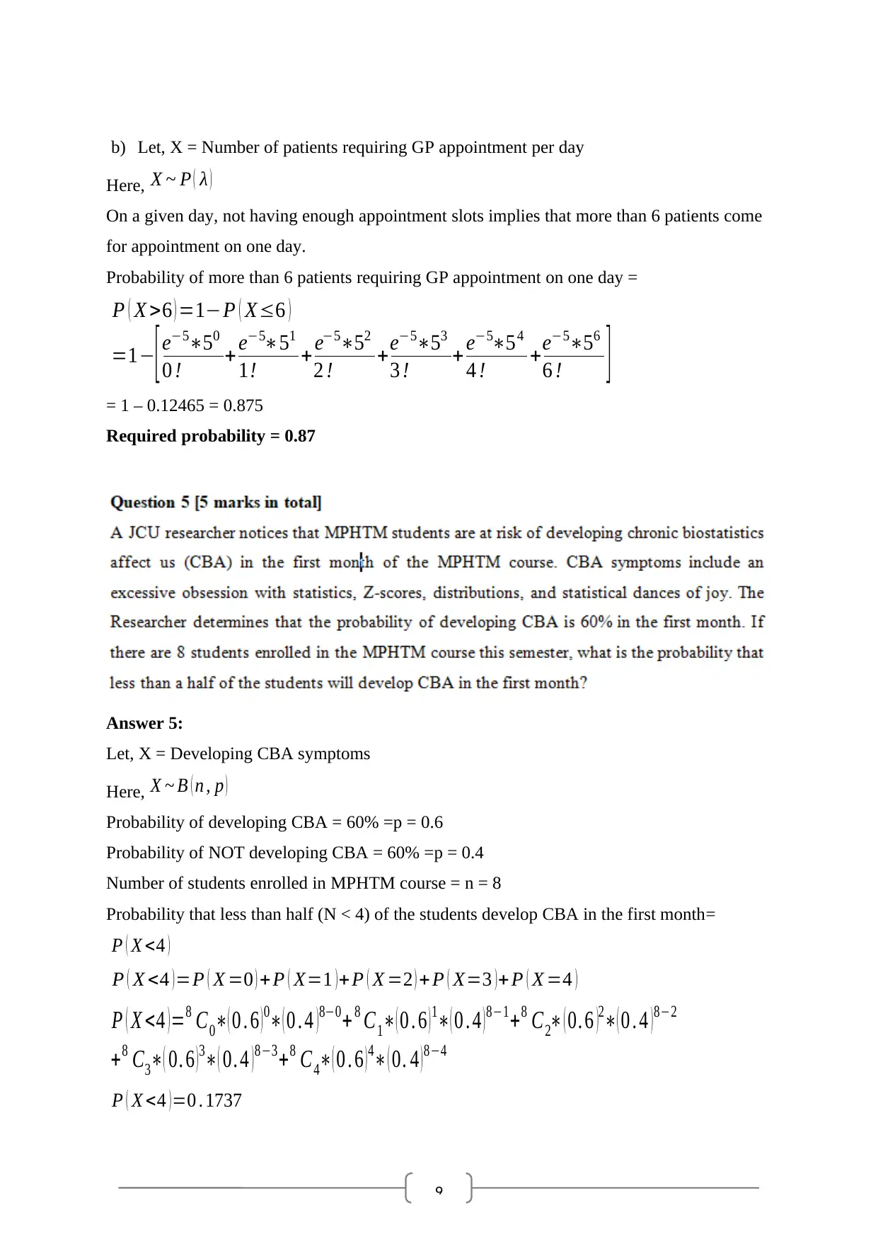
b) Let, X = Number of patients requiring GP appointment per day
Here, X ~ P ( λ )
On a given day, not having enough appointment slots implies that more than 6 patients come
for appointment on one day.
Probability of more than 6 patients requiring GP appointment on one day =
P ( X >6 ) =1−P ( X≤6 )
=1−[ e−5∗50
0 ! + e−5∗51
1! + e−5∗52
2 ! +e−5∗53
3 ! + e−5∗54
4 ! +e−5∗56
6 ! ]
= 1 – 0.12465 = 0.875
Required probability = 0.87
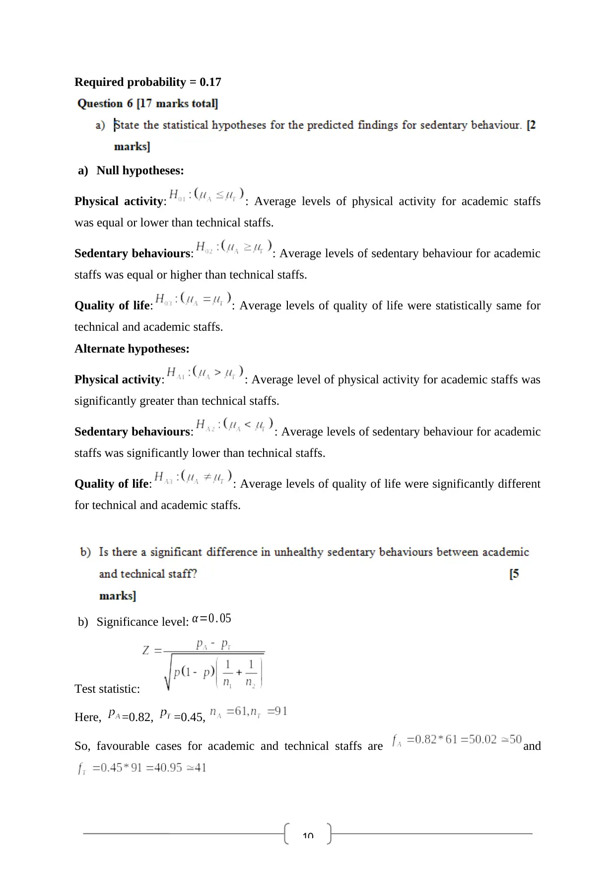
Answer 5:
Let, X = Developing CBA symptoms
Here, X ~ B ( n , p )
Probability of developing CBA = 60% =p = 0.6
Probability of NOT developing CBA = 60% =p = 0.4
Number of students enrolled in MPHTM course = n = 8
Probability that less than half (N < 4) of the students develop CBA in the first month=
P ( X <4 )
P ( X <4 ) =P ( X =0 ) + P ( X=1 ) + P ( X =2 ) + P ( X=3 ) + P ( X =4 )
P ( X <4 ) =8 C0∗( 0 . 6 ) 0∗( 0 . 4 ) 8−0+ 8 C1∗( 0 . 6 ) 1∗( 0 . 4 ) 8−1+8 C2∗ ( 0. 6 )2∗( 0 . 4 ) 8−2
+8 C3∗( 0. 6 ) 3∗( 0. 4 ) 8−3+8 C4∗( 0 . 6 ) 4∗ ( 0. 4 ) 8−4
P ( X <4 ) =0 . 1737

10
Required probability = 0.17
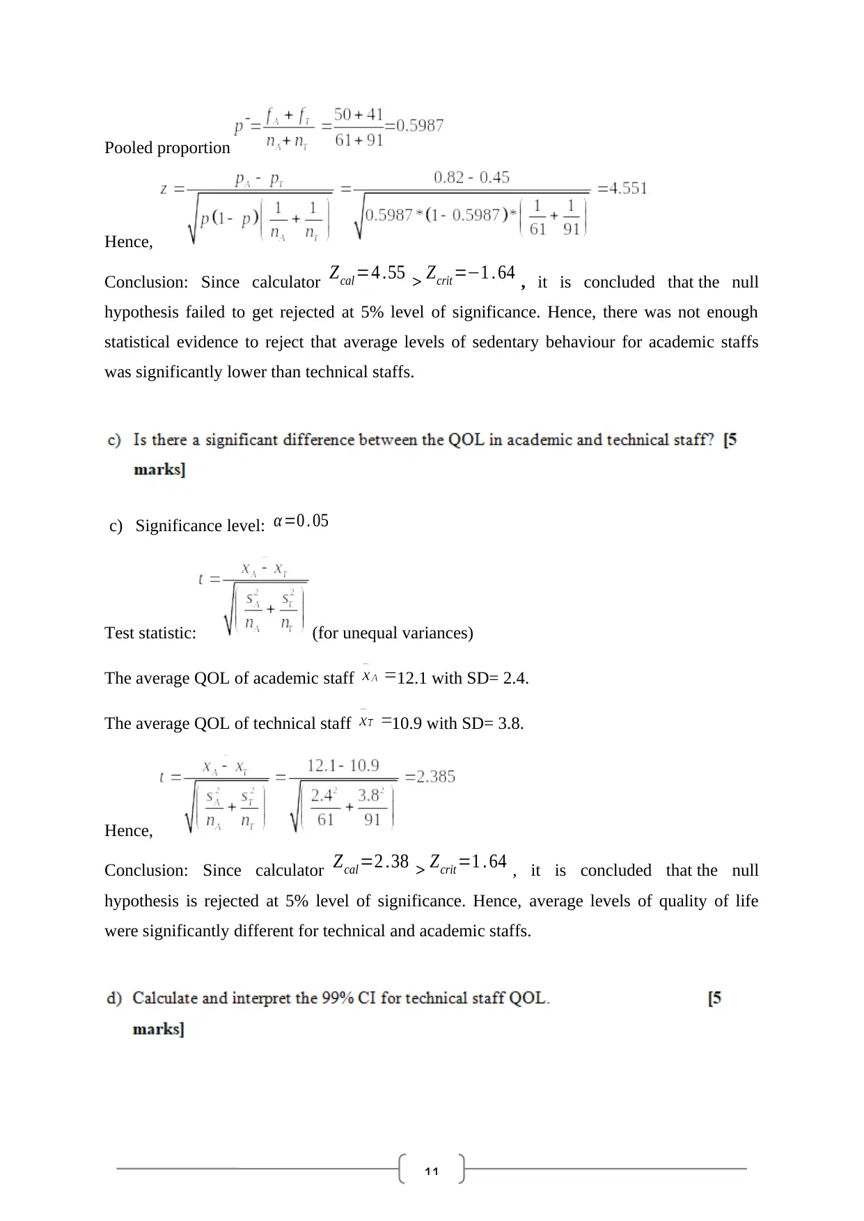
a) Null hypotheses:
Physical activity: : Average levels of physical activity for academic staffs
was equal or lower than technical staffs.
Sedentary behaviours: : Average levels of sedentary behaviour for academic
staffs was equal or higher than technical staffs.
Quality of life: : Average levels of quality of life were statistically same for
technical and academic staffs.
Alternate hypotheses:
Physical activity: : Average level of physical activity for academic staffs was
significantly greater than technical staffs.
Sedentary behaviours: : Average levels of sedentary behaviour for academic
staffs was significantly lower than technical staffs.
Quality of life: : Average levels of quality of life were significantly different
for technical and academic staffs.
b) Significance level: α=0 . 05
Test statistic:
Here, =0.82, =0.45,
So, favourable cases for academic and technical staffs are and

11
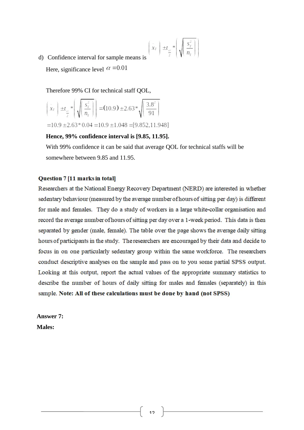
Pooled proportion
Hence,
Conclusion: Since calculator Zcal =4 .55 > Zcrit =−1 . 64 , it is concluded that the null
hypothesis failed to get rejected at 5% level of significance. Hence, there was not enough
statistical evidence to reject that average levels of sedentary behaviour for academic staffs
was significantly lower than technical staffs.
c) Significance level: α =0 . 05
Test statistic: (for unequal variances)
The average QOL of academic staff 12.1 with SD= 2.4.
The average QOL of technical staff 10.9 with SD= 3.8.
Hence,
Conclusion: Since calculator Zcal =2 .38 > Zcrit =1 . 64 , it is concluded that the null
hypothesis is rejected at 5% level of significance. Hence, average levels of quality of life
were significantly different for technical and academic staffs.

12
d) Confidence interval for sample means is
Here, significance level
Therefore 99% CI for technical staff QOL,
Hence, 99% confidence interval is [9.85, 11.95].
With 99% confidence it can be said that average QOL for technical staffs will be
somewhere between 9.85 and 11.95.
Answer 7:
Males:

13
Table 2: Frequency Distribution of hours of sitting for males
Hour (x) f x*f (x-x-bar) (x-x-bar)^2 f*(x-x-bar)^2
2 4 8 -2.86 8.16 32.65
3 2 6 -1.86 3.45 6.90
4 3 12 -0.86 0.73 2.20
5 3 15 0.14 0.02 0.06
6 2 12 1.14 1.31 2.61
7 7 49 2.14 4.59 32.15
27 21 102 -2.14 18.26 76.57
Average hours of daily sitting for males =
hours or approximately 4.86
hours.
Standard Deviation of hours of daily sitting for males =
s= √ ∑ f ( x−x
¿
)
2
∑ f = √ 76 . 57
21 =1. 91
hours.
Table 3: Cumulative frequency table for hours of sitting for males
Hour (x) f Cum.freq
2 4 4
3 2 6
4 3 9
5 3 12
6 2 14
7 7 21
27 21
N=∑ f = 21 ( odd )
Hence, Median =
21+1
2 =11 th observation.
From cumulative frequency table of hours of daily sitting for males, Median = 5 hours for
men.
Hence, First quartile =
21+1
4 =5 . 5 th observation.

14
From cumulative frequency table of hours of daily sitting for males, First quartile = 3 hours
for men.
Hence, Third quartile =
3
4∗ ( 22 ) =16 .5 th observation.
From cumulative frequency table of hours of daily sitting for males, Third quartile = 7 hours
for men.
Hence, Inter-quartile = (7-3) = 4 hours.
Summary statistics: Average of daily sitting for males was 4.86 hours with a standard
deviation of 1.91 hours. Median of daily sitting for males was 5 hours with inter-quartile
range of 4 hours. Median was slightly greater than the average. Therefore, the distribution of
daily sitting hours for males was found to be slightly left skewed.
Females:
Table 4: Frequency Distribution of hours of sitting for females
Hour (x) f x*f (x-x-bar) (x-x-bar)^2 f*(x-x-bar)^2
1 1 1 -4.71 22.18 22.18
2 3 6 -3.71 13.76 41.29
3 3 9 -2.71 7.34 22.03
4 2 8 -1.71 2.92 5.85
5 4 20 -0.71 0.50 2.02
6 1 6 0.29 0.08 0.08
7 1 7 1.29 1.66 1.66
8 1 8 2.29 5.24 5.24
9 8 72 3.29 10.82 86.59
45 24 137 -6.39 64.54 186.96
Average hours of daily sitting for females =
5.708 hours or
approximately 5.71 hours.
Standard Deviation of hours of daily sitting for females =
s= √ ∑ f ( x−x
¿
)
2
∑ f = √ 186 . 96
24 =2 .79
Hours

15
Table 5: Cumulative frequency table for hours of sitting for females
Hour (x) f Cum.freq
1 1 1
2 3 4
3 3 7
4 2 9
5 4 13
6 1 14
7 1 15
8 1 16
9 8 24
45 24
N=∑ f = 24 ( even )
Hence, Median =
24+1
2 =12. 5 th observation.
From cumulative frequency table of hours of daily sitting for males, Median = 5 hours for
females.
Hence, First quartile =
24+1
4 =6 . 25th observation.
From cumulative frequency table of hours of daily sitting for males, First quartile = 3 hours
for men.
Hence, Third quartile =
3
4∗ ( 25 ) =18 .75 th observation.
From cumulative frequency table of hours of daily sitting for males, Third quartile = 9 hours
for men.
Hence, Inter-quartile = (9-3) = 6 hours.
Summary statistics: Average of daily sitting for females was 5.71 hours with a standard
deviation of 2.79 hours. Median of daily sitting for females was 5 hours with inter-quartile
range of 6 hours. Median was lower than the average. Therefore, the distribution of daily
sitting hours for females was found to be highly right skewed.

16
Answer 8:
The p-value indicates that the treatment was not effective at 5% level of significance. But, the
treatment is noted to be effective at 10% level of significance.
Statistical significance is the probability of difference between the two groups that is likely to
be possible. If the P-value is greater than the selected Alpha level (e.g. = 0.05), it is assumed
that the possible difference observed can be explained by the variance of the sample. With a
sufficiently large sample, statistical tests are almost always significant differences. This does
not happen if there is no effect, or the total effect is zero. Thus, a very small difference, even
significant, can often be meaningless. Therefore, it is not enough for the researcher to
announce only the P-value for the analysis to fully understand the results.
The magnitude of the effect size is the most important result of a quantitative research.
Although the P-value can inform the reader if the effect exists, the P-value does not indicate
the magnitude of the effect. Both the magnitude of the impact and the expression and
interpretation of statistical significance are important results. Therefore, the extent of the
effect should be given in the study results. In fact, it is often necessary to assess the extent of
the effect before the start of the study in order to avoid the number of items that may be
needed to avoid type-II error. In other words, it is important to establish that the number of

17
subjects in the study is sufficient to have a valid power from the study that supports the null
assumptions.
Hence, the hoopla of the media based on the research results seems to be unprofessional. The
journalist needs to collect the complete results with effect size of the experiment. After that,
any conclusion will be meaningful.