Biostatistics. Name:. Institution:. A summary table of

same as this 1074722

Biostatistics
Name:
Institution:

1.
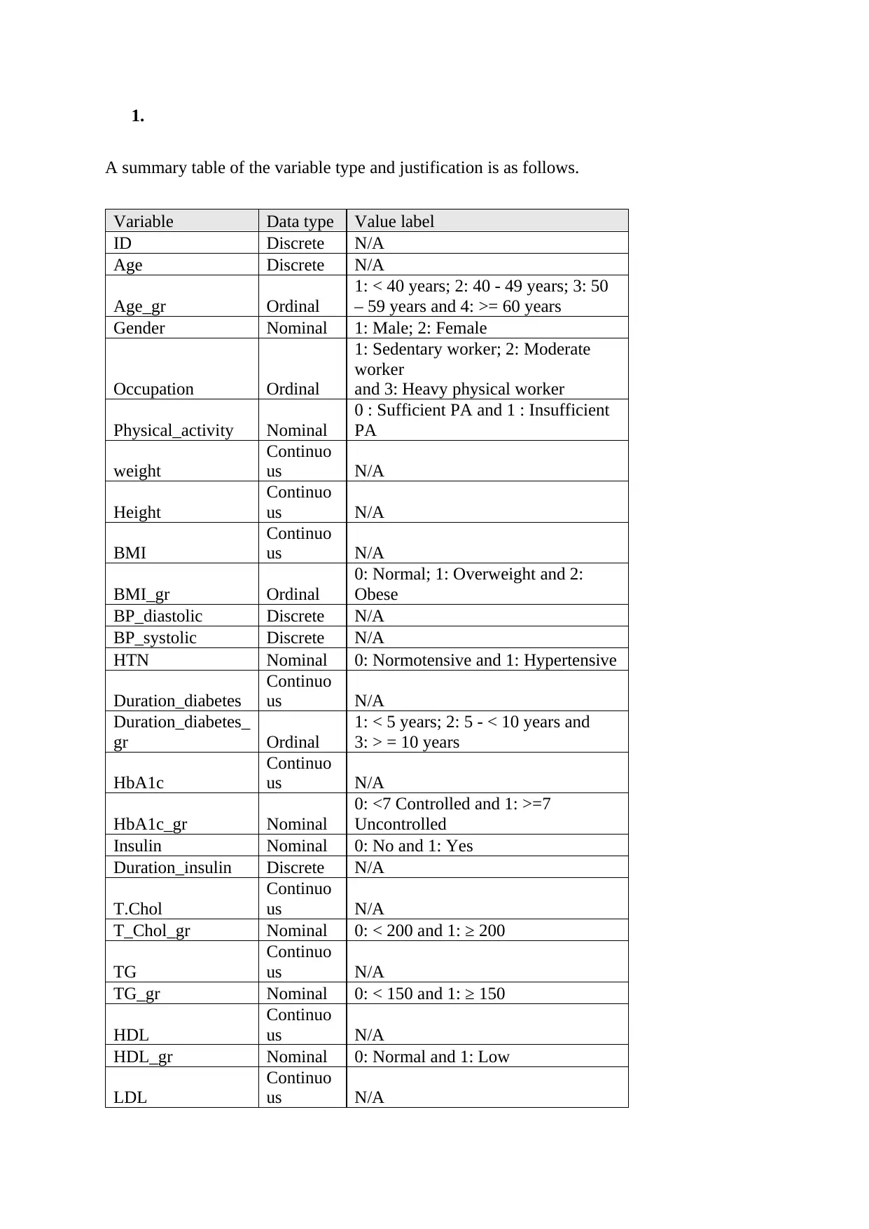
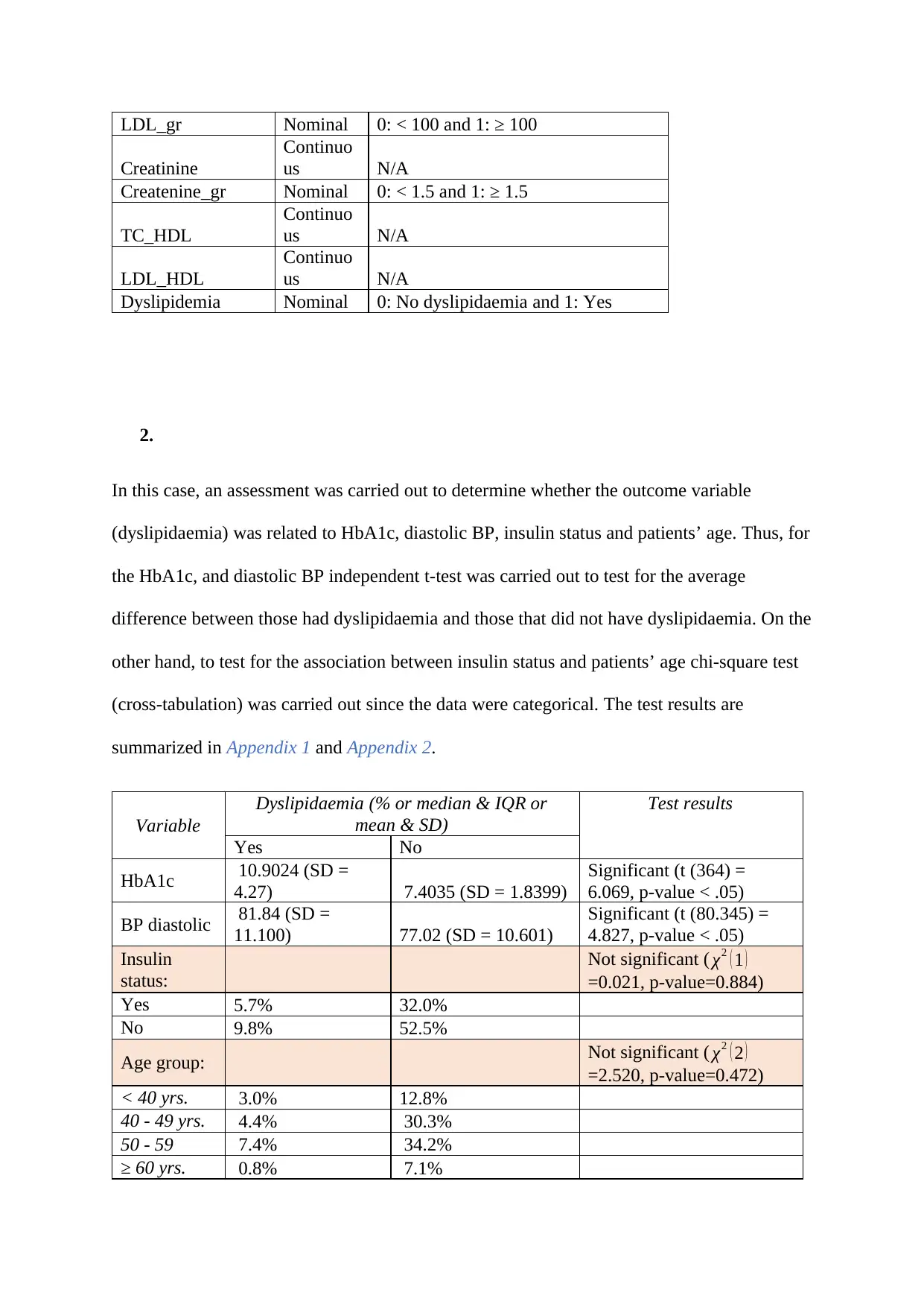
A summary table of the variable type and justification is as follows.
Variable Data type Value label
ID Discrete N/A
Age Discrete N/A
Age_gr Ordinal
1: < 40 years; 2: 40 - 49 years; 3: 50
– 59 years and 4: >= 60 years
Gender Nominal 1: Male; 2: Female
Occupation Ordinal
1: Sedentary worker; 2: Moderate
worker
and 3: Heavy physical worker
Physical_activity Nominal
0 : Sufficient PA and 1 : Insufficient
PA
weight
Continuo
us N/A
Height
Continuo
us N/A
BMI
Continuo
us N/A
BMI_gr Ordinal
0: Normal; 1: Overweight and 2:
Obese
BP_diastolic Discrete N/A
BP_systolic Discrete N/A
HTN Nominal 0: Normotensive and 1: Hypertensive
Duration_diabetes
Continuo
us N/A
Duration_diabetes_
gr Ordinal
1: < 5 years; 2: 5 - < 10 years and
3: > = 10 years
HbA1c
Continuo
us N/A
HbA1c_gr Nominal
0: <7 Controlled and 1: >=7
Uncontrolled
Insulin Nominal 0: No and 1: Yes
Duration_insulin Discrete N/A
T.Chol
Continuo
us N/A
T_Chol_gr Nominal 0: < 200 and 1: ≥ 200
TG
Continuo
us N/A
TG_gr Nominal 0: < 150 and 1: ≥ 150
HDL
Continuo
us N/A
HDL_gr Nominal 0: Normal and 1: Low
LDL
Continuo
us N/A

LDL_gr Nominal 0: < 100 and 1: ≥ 100
Creatinine
Continuo
us N/A
Createnine_gr Nominal 0: < 1.5 and 1: ≥ 1.5
TC_HDL
Continuo
us N/A
LDL_HDL
Continuo
us N/A
Dyslipidemia Nominal 0: No dyslipidaemia and 1: Yes
2.
In this case, an assessment was carried out to determine whether the outcome variable
(dyslipidaemia) was related to HbA1c, diastolic BP, insulin status and patients’ age. Thus, for
the HbA1c, and diastolic BP independent t-test was carried out to test for the average
difference between those had dyslipidaemia and those that did not have dyslipidaemia. On the
other hand, to test for the association between insulin status and patients’ age chi-square test
(cross-tabulation) was carried out since the data were categorical. The test results are
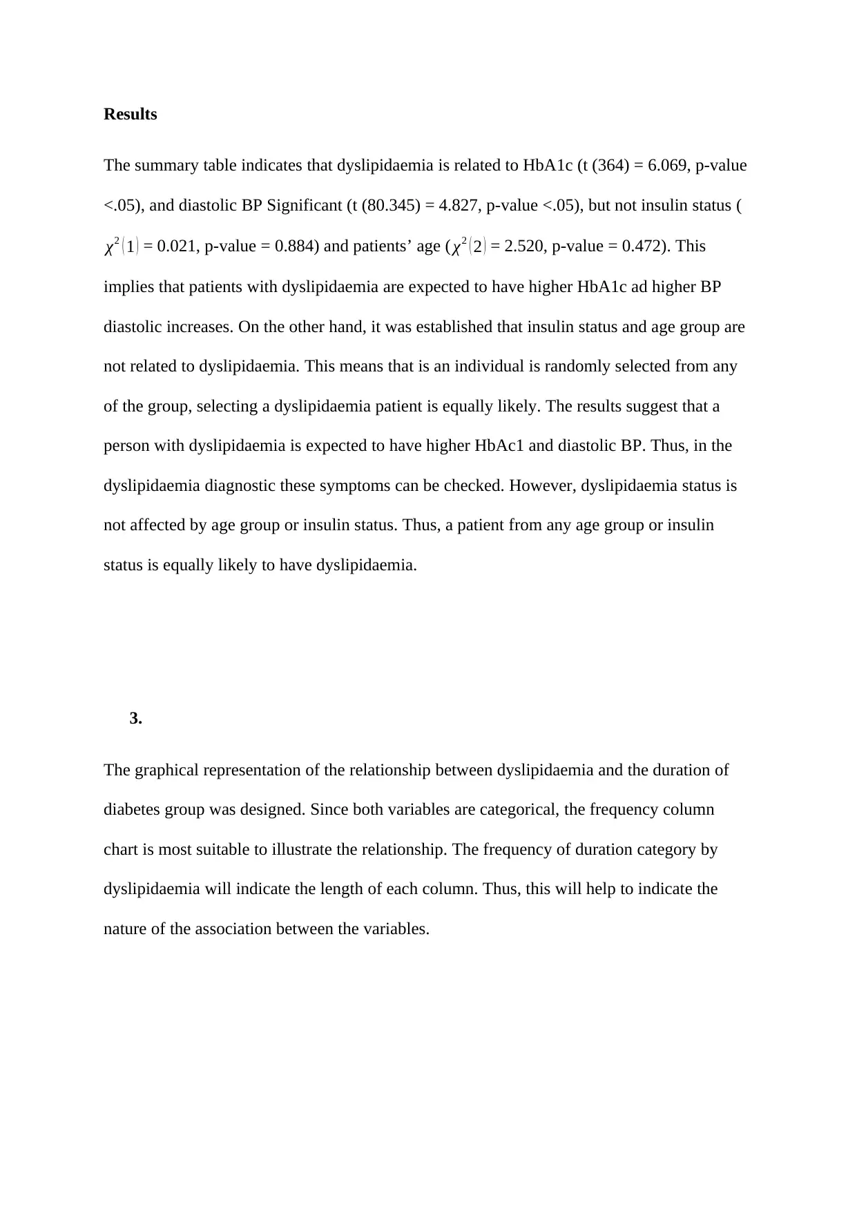
summarized in Appendix 1 and Appendix 2.
Variable
Dyslipidaemia (% or median & IQR or
mean & SD)
Test results
Yes No
HbA1c 10.9024 (SD =
4.27) 7.4035 (SD = 1.8399)
Significant (t (364) =
6.069, p-value < .05)
BP diastolic 81.84 (SD =
11.100) 77.02 (SD = 10.601)
Significant (t (80.345) =
4.827, p-value < .05)
Insulin
status:
Not significant ( χ2 ( 1 )
=0.021, p-value=0.884)
Yes 5.7% 32.0%
No 9.8% 52.5%
Age group: Not significant ( χ2 ( 2 )
=2.520, p-value=0.472)
< 40 yrs. 3.0% 12.8%
40 - 49 yrs. 4.4% 30.3%
50 - 59 7.4% 34.2%
≥ 60 yrs. 0.8% 7.1%

Results
The summary table indicates that dyslipidaemia is related to HbA1c (t (364) = 6.069, p-value
<.05), and diastolic BP Significant (t (80.345) = 4.827, p-value <.05), but not insulin status (
χ2 ( 1 ) = 0.021, p-value = 0.884) and patients’ age ( χ2 ( 2 ) = 2.520, p-value = 0.472). This
implies that patients with dyslipidaemia are expected to have higher HbA1c ad higher BP
diastolic increases. On the other hand, it was established that insulin status and age group are
not related to dyslipidaemia. This means that is an individual is randomly selected from any
of the group, selecting a dyslipidaemia patient is equally likely. The results suggest that a
person with dyslipidaemia is expected to have higher HbAc1 and diastolic BP. Thus, in the
dyslipidaemia diagnostic these symptoms can be checked. However, dyslipidaemia status is
not affected by age group or insulin status. Thus, a patient from any age group or insulin
status is equally likely to have dyslipidaemia.
3.
The graphical representation of the relationship between dyslipidaemia and the duration of
diabetes group was designed. Since both variables are categorical, the frequency column
chart is most suitable to illustrate the relationship. The frequency of duration category by
dyslipidaemia will indicate the length of each column. Thus, this will help to indicate the
nature of the association between the variables.

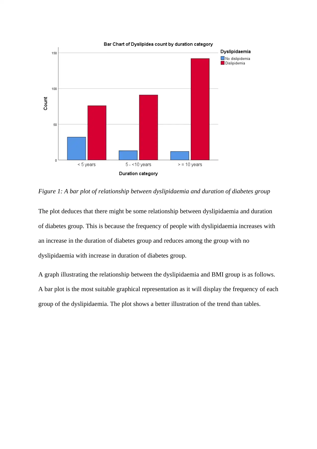
Figure 1: A bar plot of relationship between dyslipidaemia and duration of diabetes group
The plot deduces that there might be some relationship between dyslipidaemia and duration
of diabetes group. This is because the frequency of people with dyslipidaemia increases with
an increase in the duration of diabetes group and reduces among the group with no
dyslipidaemia with increase in duration of diabetes group.
A graph illustrating the relationship between the dyslipidaemia and BMI group is as follows.
A bar plot is the most suitable graphical representation as it will display the frequency of each
group of the dyslipidaemia. The plot shows a better illustration of the trend than tables.

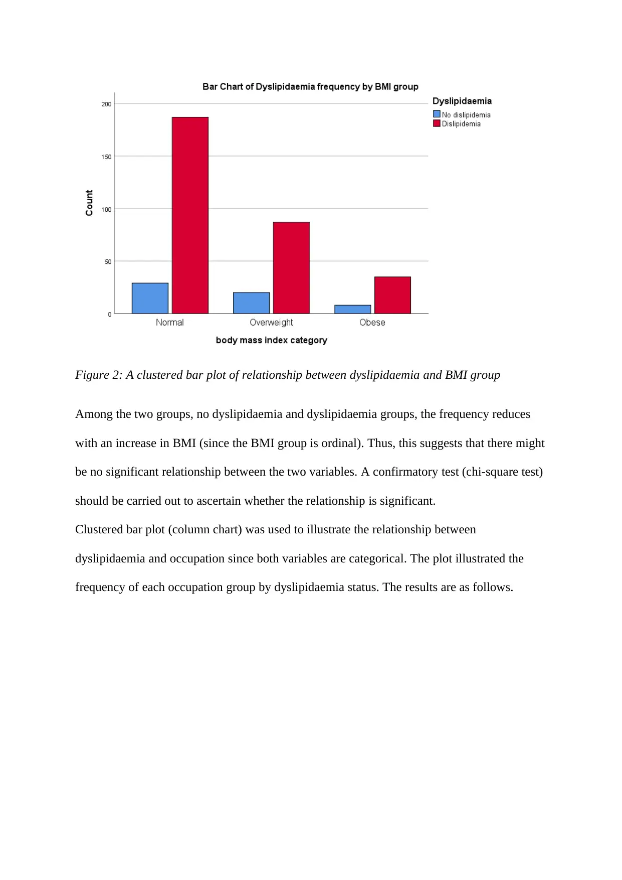
Figure 2: A clustered bar plot of relationship between dyslipidaemia and BMI group
Among the two groups, no dyslipidaemia and dyslipidaemia groups, the frequency reduces
with an increase in BMI (since the BMI group is ordinal). Thus, this suggests that there might
be no significant relationship between the two variables. A confirmatory test (chi-square test)
should be carried out to ascertain whether the relationship is significant.
Clustered bar plot (column chart) was used to illustrate the relationship between
dyslipidaemia and occupation since both variables are categorical. The plot illustrated the
frequency of each occupation group by dyslipidaemia status. The results are as follows.

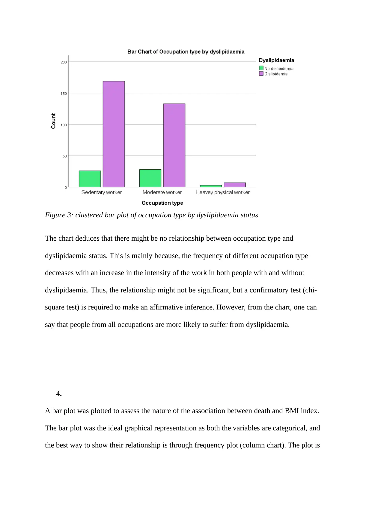
Figure 3: clustered bar plot of occupation type by dyslipidaemia status
The chart deduces that there might be no relationship between occupation type and
dyslipidaemia status. This is mainly because, the frequency of different occupation type
decreases with an increase in the intensity of the work in both people with and without
dyslipidaemia. Thus, the relationship might not be significant, but a confirmatory test (chi-
square test) is required to make an affirmative inference. However, from the chart, one can
say that people from all occupations are more likely to suffer from dyslipidaemia.
4.
A bar plot was plotted to assess the nature of the association between death and BMI index.
The bar plot was the ideal graphical representation as both the variables are categorical, and
the best way to show their relationship is through frequency plot (column chart). The plot is

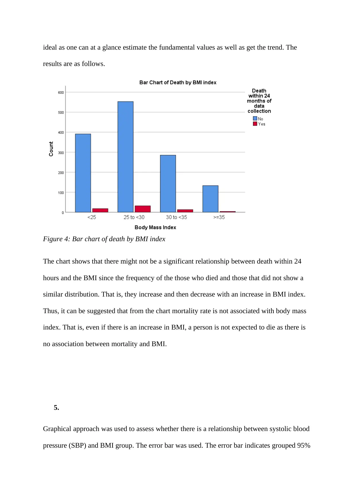
ideal as one can at a glance estimate the fundamental values as well as get the trend. The
results are as follows.
Figure 4: Bar chart of death by BMI index
The chart shows that there might not be a significant relationship between death within 24
hours and the BMI since the frequency of the those who died and those that did not show a
similar distribution. That is, they increase and then decrease with an increase in BMI index.
Thus, it can be suggested that from the chart mortality rate is not associated with body mass
index. That is, even if there is an increase in BMI, a person is not expected to die as there is
no association between mortality and BMI.
5.
Graphical approach was used to assess whether there is a relationship between systolic blood
pressure (SBP) and BMI group. The error bar was used. The error bar indicates grouped 95%

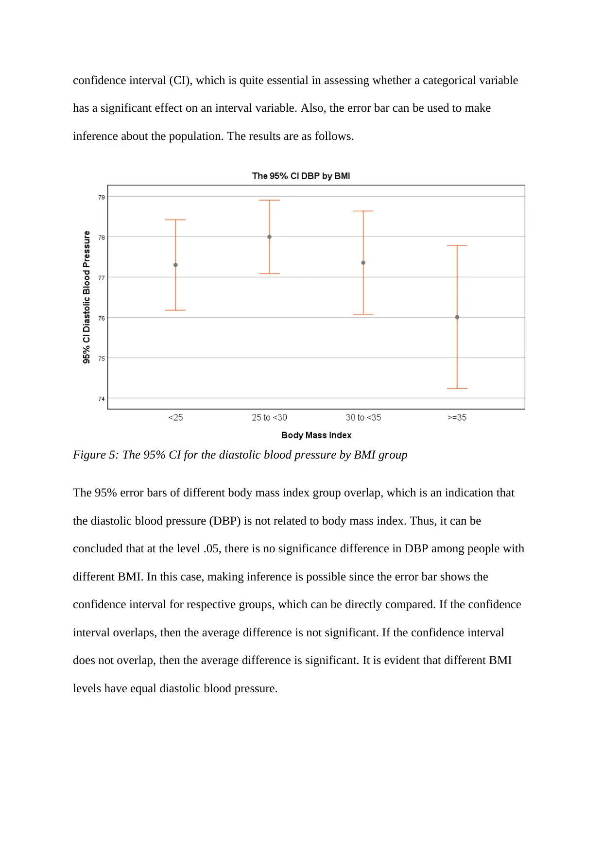
confidence interval (CI), which is quite essential in assessing whether a categorical variable
has a significant effect on an interval variable. Also, the error bar can be used to make
inference about the population. The results are as follows.
Figure 5: The 95% CI for the diastolic blood pressure by BMI group
The 95% error bars of different body mass index group overlap, which is an indication that
the diastolic blood pressure (DBP) is not related to body mass index. Thus, it can be
concluded that at the level .05, there is no significance difference in DBP among people with
different BMI. In this case, making inference is possible since the error bar shows the
confidence interval for respective groups, which can be directly compared. If the confidence
interval overlaps, then the average difference is not significant. If the confidence interval
does not overlap, then the average difference is significant. It is evident that different BMI
levels have equal diastolic blood pressure.

6.
T-test was used to determine whether there is a significant difference in the average SBP,
DBP, and CHL among the patients who received drug-X and those that did not receive. This
approach was ideal as the dependent variables (SBP, DBP, and CHL) were numerical
variables and the independent variable had two categories. The two groups averages the
difference is computed and tested if it is statistically different.
Variable
Summary statistics p-value 95% CI (where
appropriate)
Yes Drug-X No Drug-X
Systolic blood
pressure
140.05 (SD
= 19.571) 141.03 (SD = 19.020) .369 (-3.112, 1.157)
Diastolic blood
pressure
77.42 (SD
= 11.375) 77.57 (SD = 10.993) .817 (-1.384, 1.092)
Cholesterol level
176.6093
(SD =
37.4467)
181.5961 (SD =
37.23082) .018
(-9.09954,
-.87401)
The results show that SBP and DBP are not significantly different among patients that receive
the drug-X treatment. On the other hand, the cholesterol level is significantly different
between the patients that received the drug-X treatment. Those that do receive the treatment
has a lower average cholesterol level. Appendix 3 has complete summary statistics. The
confidence interval that contains zero means that the average difference is not statistically
different. This is the case, for the SBP (95% CI = (-3.112, 1.157)) and DBP (95% CI = (-
1.384, 1.092)). On the other hand, the cholesterol level confidence interval does not contain
zero, which means that the average difference between those that took drug-X and those that
did was significant. Thus, it can be concluded that patients taking the drug-X has a
significantly different cholesterol level, and the DBP and SBP are not significantly different.
7.

The assessment of whether SBP average is significantly different among the three BMI
categories (BMI <25, BMI 25 to <30 and BMI ≥ 30kg/m2) was carried out using the one-way
ANOVA test. This is because the grouping variable has three independent categories, and the
dependent variable is numerical in nature. First, a new variable for BMI is recoded so that the
three categories can be formed since the first variable had four independent categories {0 =
BMI <20, 1 = BMI 25 to < 30, 2 = BMI ≥ 30}. The test was performed at the level .05, and
the hypothesis was that at least one of the BMI group has a significantly different systolic
blood pressure.
H0: All the BMI group has equal systolic blood pressure.
Ha: at least one of the BMI group has a significantly different systolic blood pressure.
The null hypothesis is rejected when the p-value of the test is less than .05.
The test results are as follows.
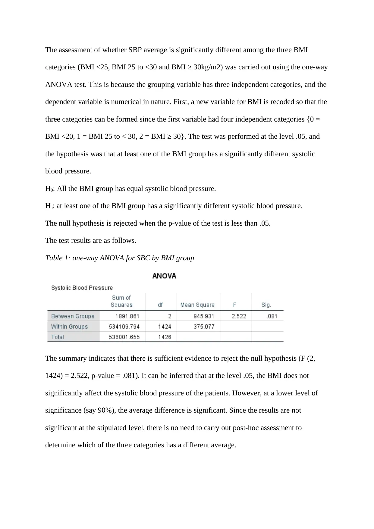
Table 1: one-way ANOVA for SBC by BMI group
The summary indicates that there is sufficient evidence to reject the null hypothesis (F (2,
1424) = 2.522, p-value = .081). It can be inferred that at the level .05, the BMI does not
significantly affect the systolic blood pressure of the patients. However, at a lower level of
significance (say 90%), the average difference is significant. Since the results are not
significant at the stipulated level, there is no need to carry out post-hoc assessment to
determine which of the three categories has a different average.

Appendix
Appendix 1: Q2 t-test
Appendix 2: Q2 chi-square

Appendix 3: Q6 t-test
Appendix 4: Q 7 ANOVA test