Critical Review of a Biostatistics Study and Descriptive Analysis Findings

This article presents a critical review of a biostatistics study based on STROBE guidelines and findings of descriptive analysis. It includes summary statistics, histogram, boxplot, and regression analysis results.

Introduction to Biostatistics
Student name:
Student number:
Lecturer name:

Task 1:
Critical review of the paper
Strobe 10 Study size
The sample size used for this study was 775. This is a big enough sample size to generate
statistically significant results. The authors did clearly mention about the sample size they
used hence the item on strobe 10 is fully conformed with.
Strobe 12 Statistical methods
a) Description of statistical methodologies used
This item needs to conform to strobe item 12a. The authors are supposed to document the
various statistical methodologies they employed in the study as well as the manner in which
control for confounding was done. Even though the authors did present the results, they failed
to highlight the descriptive statistics as well as the inferential statistics used in the study.
b) Description of any methods used to examine subgroups and interactions
Despite presenting results on subgroups in all the results they presented, the authors failed to
document or highlight the methodology used to analyse the subgroups and as such the authors
did not comply with strobe 12b on subgroup.
c) Explanation on how missing data were addressed
In the entire report presented by the authors, there was no single mention on how missing
data issue was dealt with even though the presence of missing data could be traced in some of
the presented results. This means that the authors did not adhere to the use of item 12c of the
strobe.
d) Description of the sampling technique-cross-sectional study

A cross-section design was used for this study. The procedure of sampling was well
documented and presented by the authors. This clearly addressed the strobe 12d item. The
only information the authors failed to explain was why they decided to the data collection on
only some specific selected days.
e) Description of any sensitivity analysis performed
In this study, there was no sensitivity analysis that was performed neither was it mentioned
by the authors as such item on strobe 12e was not conformed with.
Strobe 13: Participants
a) Report on participants
There was mention of the kind of participants recruited in the study. So the authors complied
with item 13a.
b) Reasons for non-participant at each stage
There was violation of item on strobe 13b. The authors did not highlight the reasons for non-
participant at each and every stage.
c) Consider use of a flow diagram
The authors did not present a flow diagram for the responses hence they failed to comply
with item on strobe 13c.
Strobe 14 Descriptive data
a) Participants characteristics
The authors clearly gave the demographic characteristics of the participants in table 1. This
complies with item on strobe 14a.

b) Indicate number of participants with missing data for each variable of interest
No mention on number of participants with missing data for each variable of interest hence
failure to comply with item on strobe 14b.
c) Cohort study: description of follow-up time.
This being a cross-sectional study it did not require any follow up with the participants and so
though Strobe 14c is missing it is irrelevant in this study.
Strobe 15
Cross-sectional study—outcome measures
There is mention of the findings hence we can say that strobe 15 was complied with.
Strobe 16 Main results
a) Unadjusted estimates
The authors did not give the adjusted estimates or even the confounder-adjusted
estimates. In fact they did even mention anything to do with confounders in the first
place.
b) Report category boundaries when continuous variables were categorised
The authors complied with item on strobe 16b by fully describing the boundaries used to
convert the numeric variables in the study.
c) Report on absolute risk
No mention on the absolute risk hence failure to comply with item on strobe 16c.
Strobe 17 Other analyses done

The authors failed to mention the analysis used. Evan though they presented the results they
did not mention on the statistical analysis performed hence failed to comply with item on
strobe 17.

Question 2:
Present the findings of your descriptive analyses
Answer
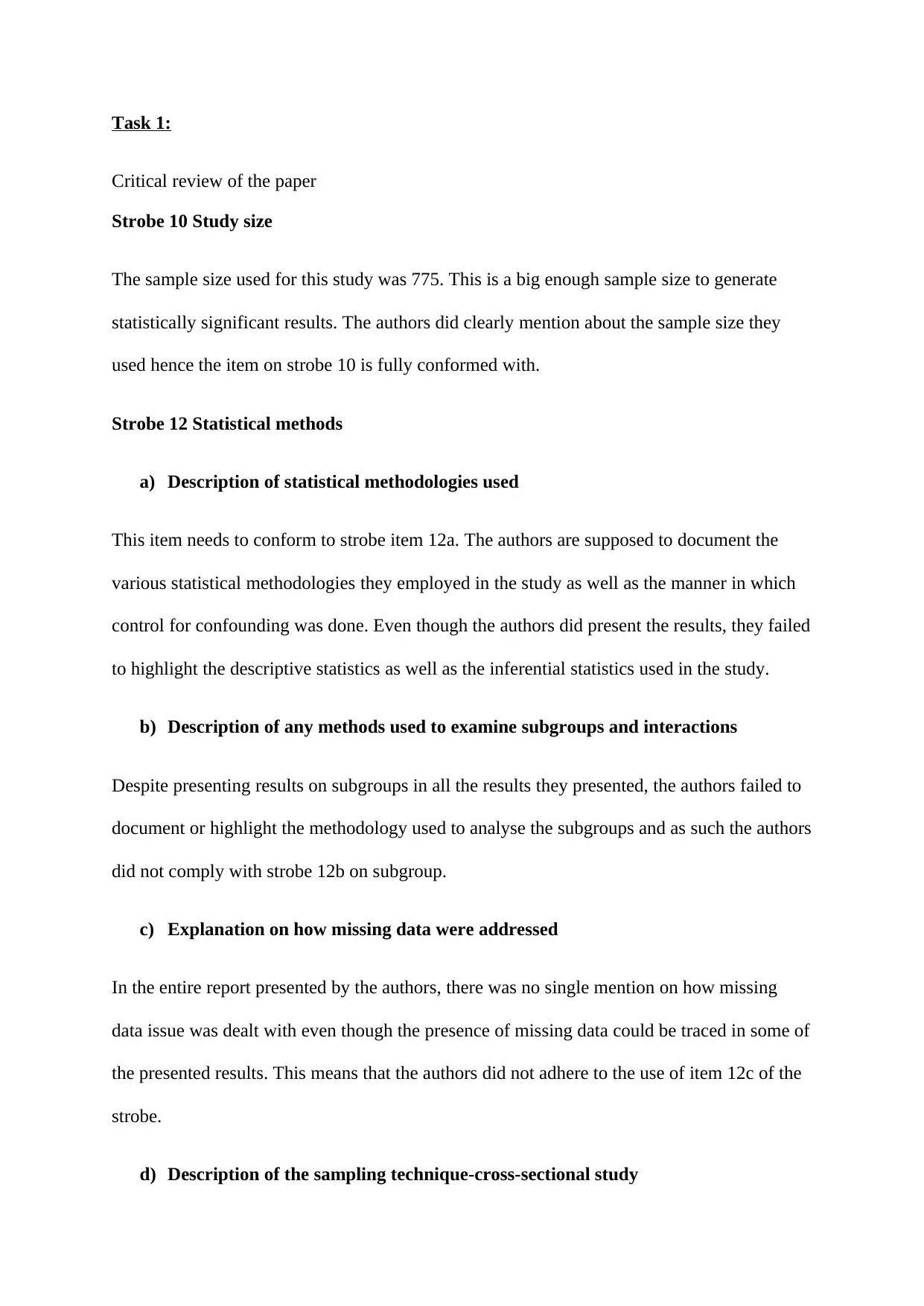
Summary statistics
The summary statistics for the numeric variables is presented below;
As can be seen, the average number of activities was found
to be 7.236 with the maximum number of activities held in
the past one month being 12 and the minimum being 2. The
average self-reported sedentary hours per week was 10.44
with the highest score being 20 and the lowest core being
4.10. For the MVPA, the average was found to be 3.929 with the minimum and maximum
values being 0.4 and 22.70 respectively.
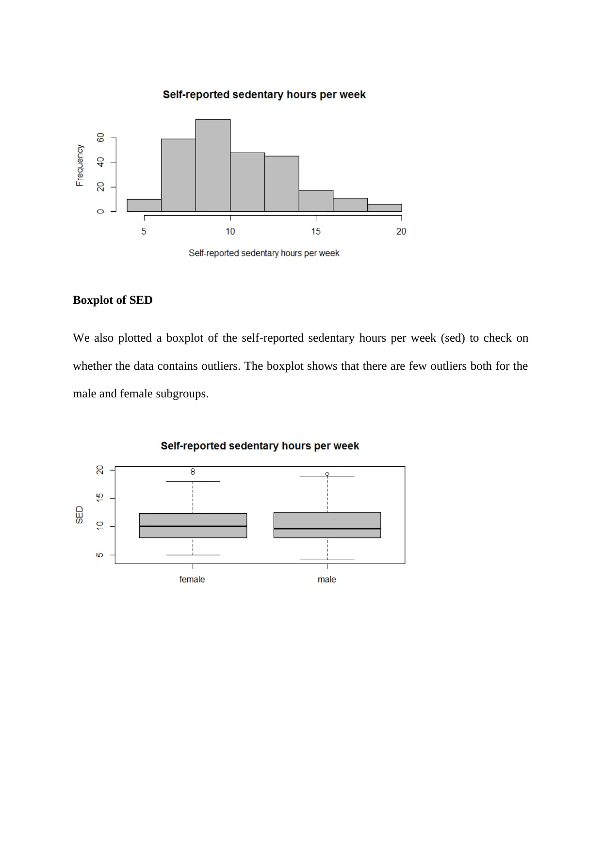
Histogram of the SED
In the figure below, we present the histogram of the self-reported sedentary hours per week
(sed). The figure clearly shows that the data is not normally distributed but is rather skewed
to the right (longer tail to the right).
> summary(newdata)
activities sed
MVPA
Min. : 2.000 Min. :
4.10 Min. : 0.400
1st Qu.: 6.000 1st Qu.:
8.00 1st Qu.: 1.600
Median : 7.000
Median : 9.80 Median :
2.900
Mean : 7.236
Mean :10.44 Mean :
3.929
3rd Qu.: 9.000 3rd
Qu.:12.30 3rd Qu.:
5.100
Max. :12.000
Max. :20.00
Max. :22.700

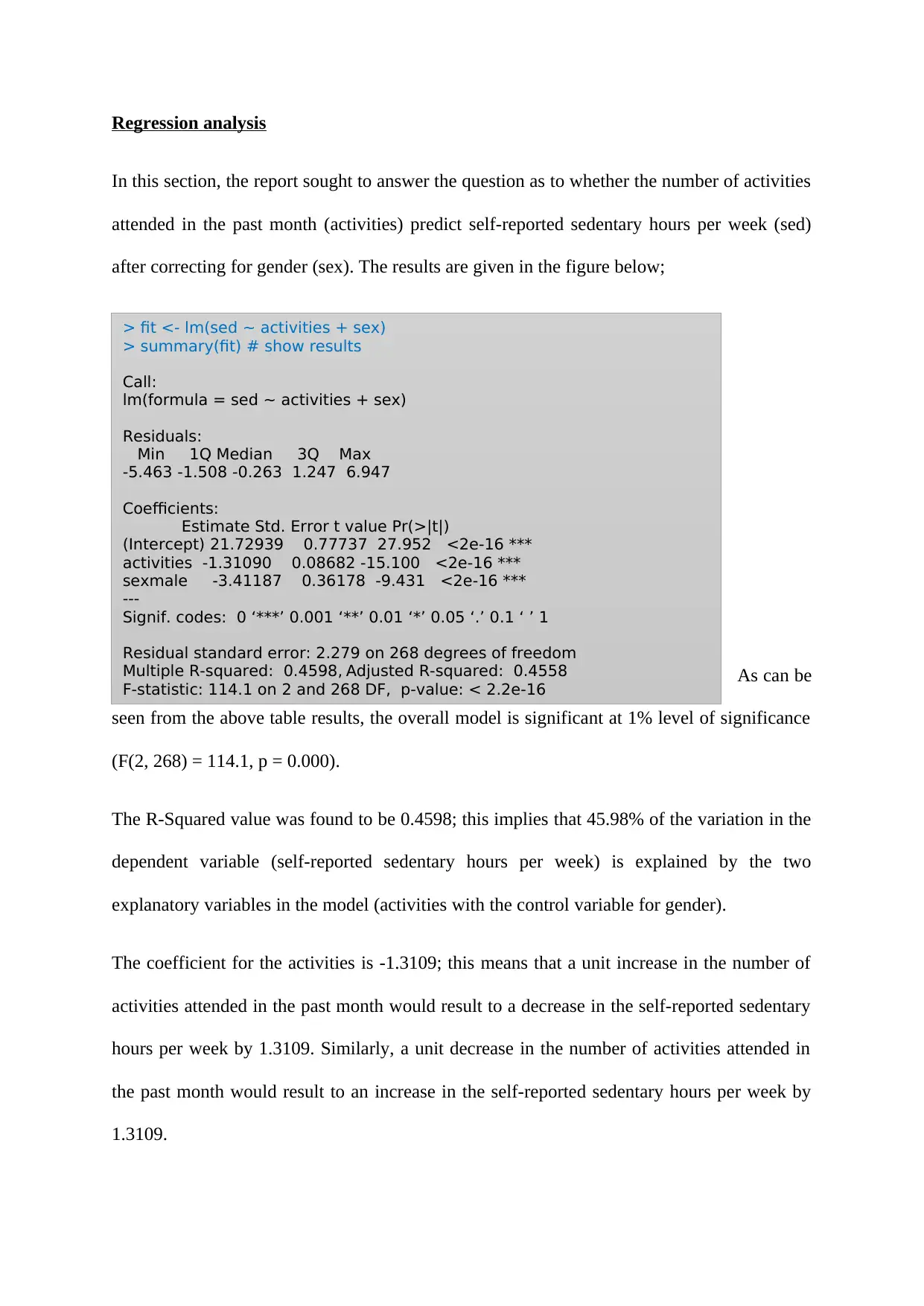
Boxplot of SED
We also plotted a boxplot of the self-reported sedentary hours per week (sed) to check on
whether the data contains outliers. The boxplot shows that there are few outliers both for the
male and female subgroups.

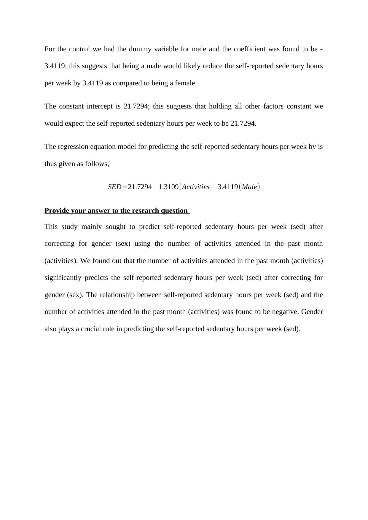
Regression analysis
In this section, the report sought to answer the question as to whether the number of activities
attended in the past month (activities) predict self-reported sedentary hours per week (sed)
after correcting for gender (sex). The results are given in the figure below;
As can be
seen from the above table results, the overall model is significant at 1% level of significance
(F(2, 268) = 114.1, p = 0.000).
The R-Squared value was found to be 0.4598; this implies that 45.98% of the variation in the
dependent variable (self-reported sedentary hours per week) is explained by the two
explanatory variables in the model (activities with the control variable for gender).
The coefficient for the activities is -1.3109; this means that a unit increase in the number of
activities attended in the past month would result to a decrease in the self-reported sedentary
hours per week by 1.3109. Similarly, a unit decrease in the number of activities attended in
the past month would result to an increase in the self-reported sedentary hours per week by
1.3109.
> fit <- lm(sed ~ activities + sex)
> summary(fit) # show results
Call:
lm(formula = sed ~ activities + sex)
Residuals:
Min 1Q Median 3Q Max
-5.463 -1.508 -0.263 1.247 6.947
Coefficients:
Estimate Std. Error t value Pr(>|t|)
(Intercept) 21.72939 0.77737 27.952 <2e-16 ***
activities -1.31090 0.08682 -15.100 <2e-16 ***
sexmale -3.41187 0.36178 -9.431 <2e-16 ***
---
Signif. codes: 0 ‘***’ 0.001 ‘**’ 0.01 ‘*’ 0.05 ‘.’ 0.1 ‘ ’ 1
Residual standard error: 2.279 on 268 degrees of freedom
Multiple R-squared: 0.4598, Adjusted R-squared: 0.4558
F-statistic: 114.1 on 2 and 268 DF, p-value: < 2.2e-16

For the control we had the dummy variable for male and the coefficient was found to be -
3.4119; this suggests that being a male would likely reduce the self-reported sedentary hours
per week by 3.4119 as compared to being a female.
The constant intercept is 21.7294; this suggests that holding all other factors constant we
would expect the self-reported sedentary hours per week to be 21.7294.
The regression equation model for predicting the self-reported sedentary hours per week by is
thus given as follows;
SED=21.7294−1.3109 ( Activities ) −3.4119(Male)
Provide your answer to the research question
This study mainly sought to predict self-reported sedentary hours per week (sed) after
correcting for gender (sex) using the number of activities attended in the past month
(activities). We found out that the number of activities attended in the past month (activities)
significantly predicts the self-reported sedentary hours per week (sed) after correcting for
gender (sex). The relationship between self-reported sedentary hours per week (sed) and the
number of activities attended in the past month (activities) was found to be negative. Gender
also plays a crucial role in predicting the self-reported sedentary hours per week (sed).

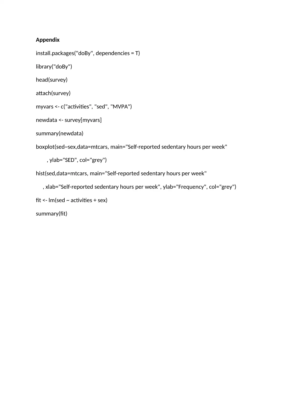
Appendix
install.packages("doBy", dependencies = T)
library("doBy")
head(survey)
attach(survey)
myvars <- c("activities", "sed", "MVPA")
newdata <- survey[myvars]
summary(newdata)
boxplot(sed~sex,data=mtcars, main="Self-reported sedentary hours per week"
, ylab="SED", col="grey")
hist(sed,data=mtcars, main="Self-reported sedentary hours per week"
, xlab="Self-reported sedentary hours per week", ylab="Frequency", col="grey")
fit <- lm(sed ~ activities + sex)
summary(fit)