Building Mathematics

This document provides solutions for various scenarios and equations in Building Mathematics. It covers topics such as area of rectangle, daily forfeit and original contract, dimensional parameters, fuel consumption, units of lift, arithmetic progression sequence, geometric progression sequence, and equations for x.

Building Mathematics 1
BUILDING MATHEMATICS
Name
Course
Professor
University
City/state
Date

Building Mathematics 2
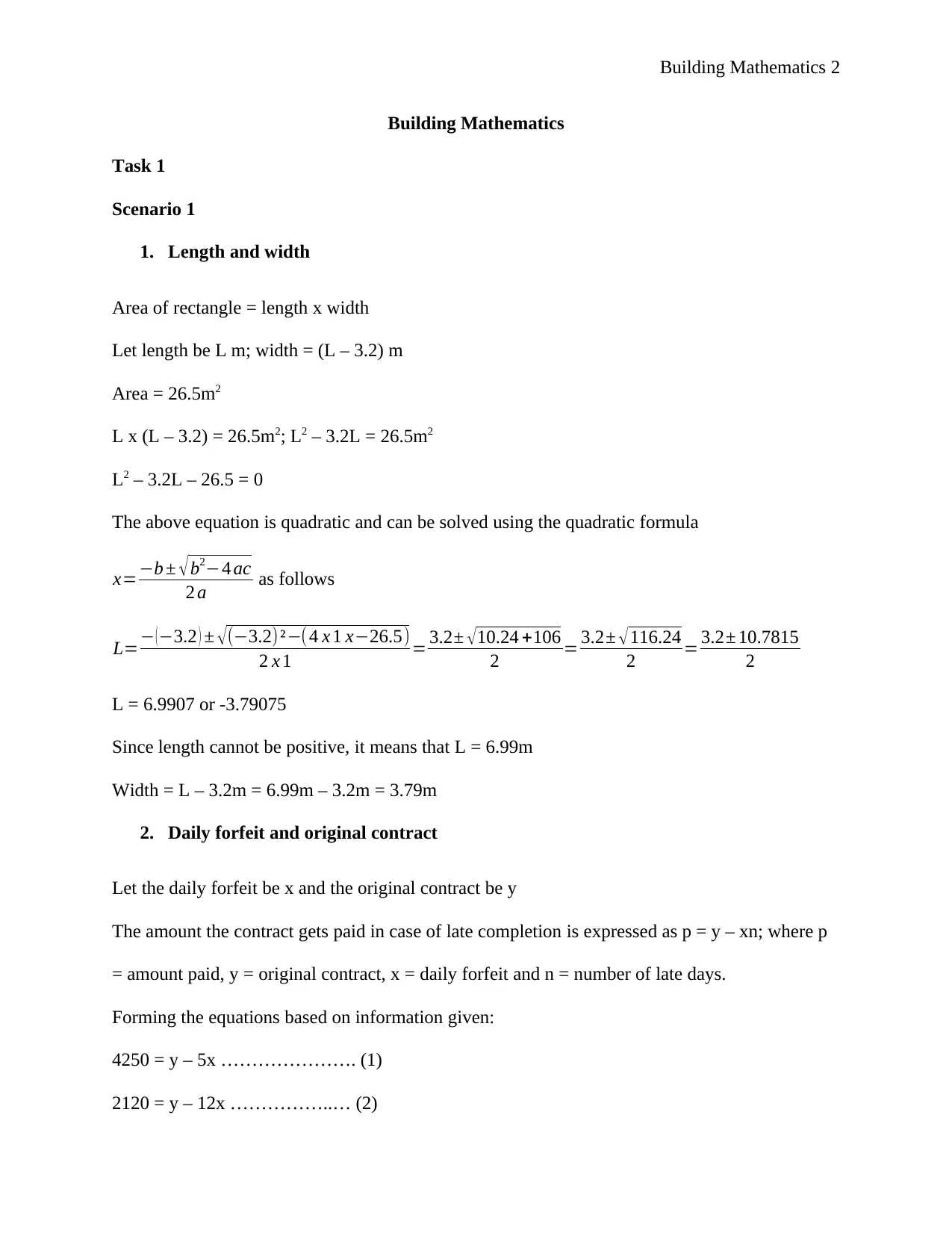
Building Mathematics
Task 1
Scenario 1
1. Length and width
Area of rectangle = length x width
Let length be L m; width = (L – 3.2) m
Area = 26.5m2
L x (L – 3.2) = 26.5m2; L2 – 3.2L = 26.5m2
L2 – 3.2L – 26.5 = 0
The above equation is quadratic and can be solved using the quadratic formula
x=−b ± √ b2−4 ac
2 a as follows
L=− (−3.2 ) ± √(−3.2)²−(4 x 1 x−26.5)
2 x 1 = 3.2± √10.24 +106
2 = 3.2± √116.24
2 = 3.2± 10.7815
2
L = 6.9907 or -3.79075
Since length cannot be positive, it means that L = 6.99m
Width = L – 3.2m = 6.99m – 3.2m = 3.79m
2. Daily forfeit and original contract
Let the daily forfeit be x and the original contract be y
The amount the contract gets paid in case of late completion is expressed as p = y – xn; where p
= amount paid, y = original contract, x = daily forfeit and n = number of late days.
Forming the equations based on information given:
4250 = y – 5x …………………. (1)
2120 = y – 12x ……………..… (2)

Building Mathematics 3
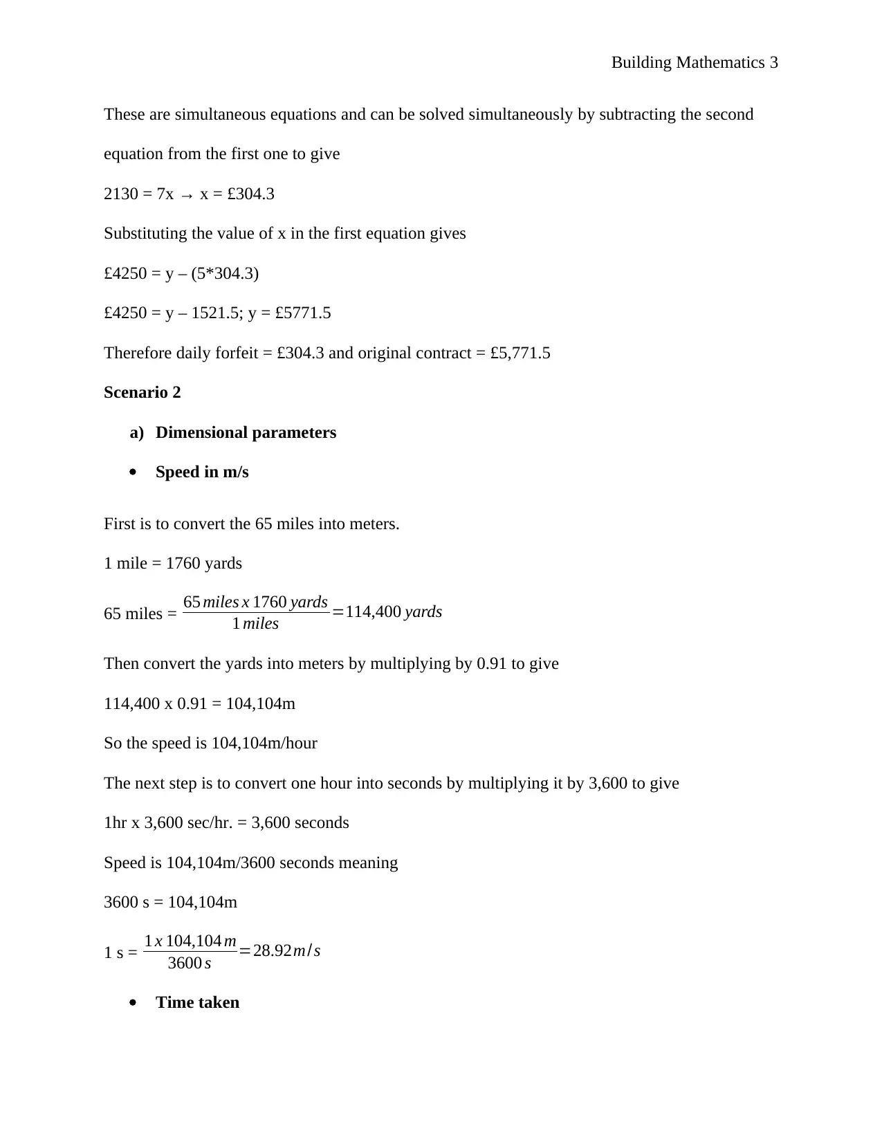
These are simultaneous equations and can be solved simultaneously by subtracting the second
equation from the first one to give
2130 = 7x → x = £304.3
Substituting the value of x in the first equation gives
£4250 = y – (5*304.3)
£4250 = y – 1521.5; y = £5771.5
Therefore daily forfeit = £304.3 and original contract = £5,771.5
Scenario 2
a) Dimensional parameters
 Speed in m/s
First is to convert the 65 miles into meters.
1 mile = 1760 yards
65 miles = 65 miles x 1760 yards
1 miles =114,400 yards
Then convert the yards into meters by multiplying by 0.91 to give
114,400 x 0.91 = 104,104m
So the speed is 104,104m/hour
The next step is to convert one hour into seconds by multiplying it by 3,600 to give
1hr x 3,600 sec/hr. = 3,600 seconds
Speed is 104,104m/3600 seconds meaning
3600 s = 104,104m
1 s = 1 x 104,104 m
3600 s =28.92m/s
 Time taken

Building Mathematics 4
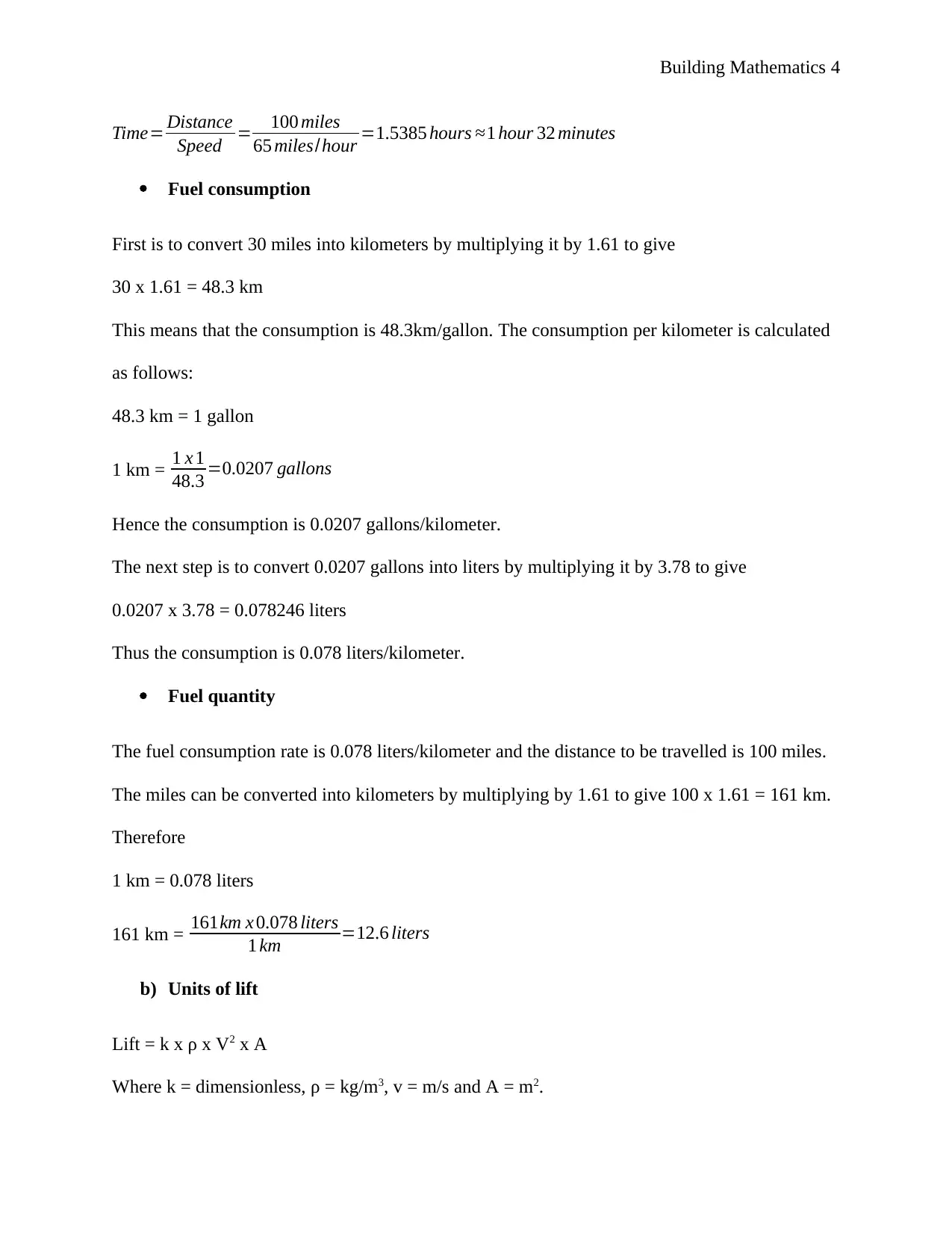
Time= Distance
Speed = 100 miles
65 miles/hour =1.5385 hours ≈1 hour 32 minutes
 Fuel consumption
First is to convert 30 miles into kilometers by multiplying it by 1.61 to give
30 x 1.61 = 48.3 km
This means that the consumption is 48.3km/gallon. The consumption per kilometer is calculated
as follows:
48.3 km = 1 gallon
1 km = 1 x 1
48.3 =0.0207 gallons
Hence the consumption is 0.0207 gallons/kilometer.
The next step is to convert 0.0207 gallons into liters by multiplying it by 3.78 to give
0.0207 x 3.78 = 0.078246 liters
Thus the consumption is 0.078 liters/kilometer.
 Fuel quantity
The fuel consumption rate is 0.078 liters/kilometer and the distance to be travelled is 100 miles.
The miles can be converted into kilometers by multiplying by 1.61 to give 100 x 1.61 = 161 km.
Therefore
1 km = 0.078 liters
161 km = 161km x 0.078 liters
1 km =12.6 liters
b) Units of lift
Lift = k x ρ x V2 x A
Where k = dimensionless, ρ = kg/m3, v = m/s and A = m2.

Building Mathematics 5
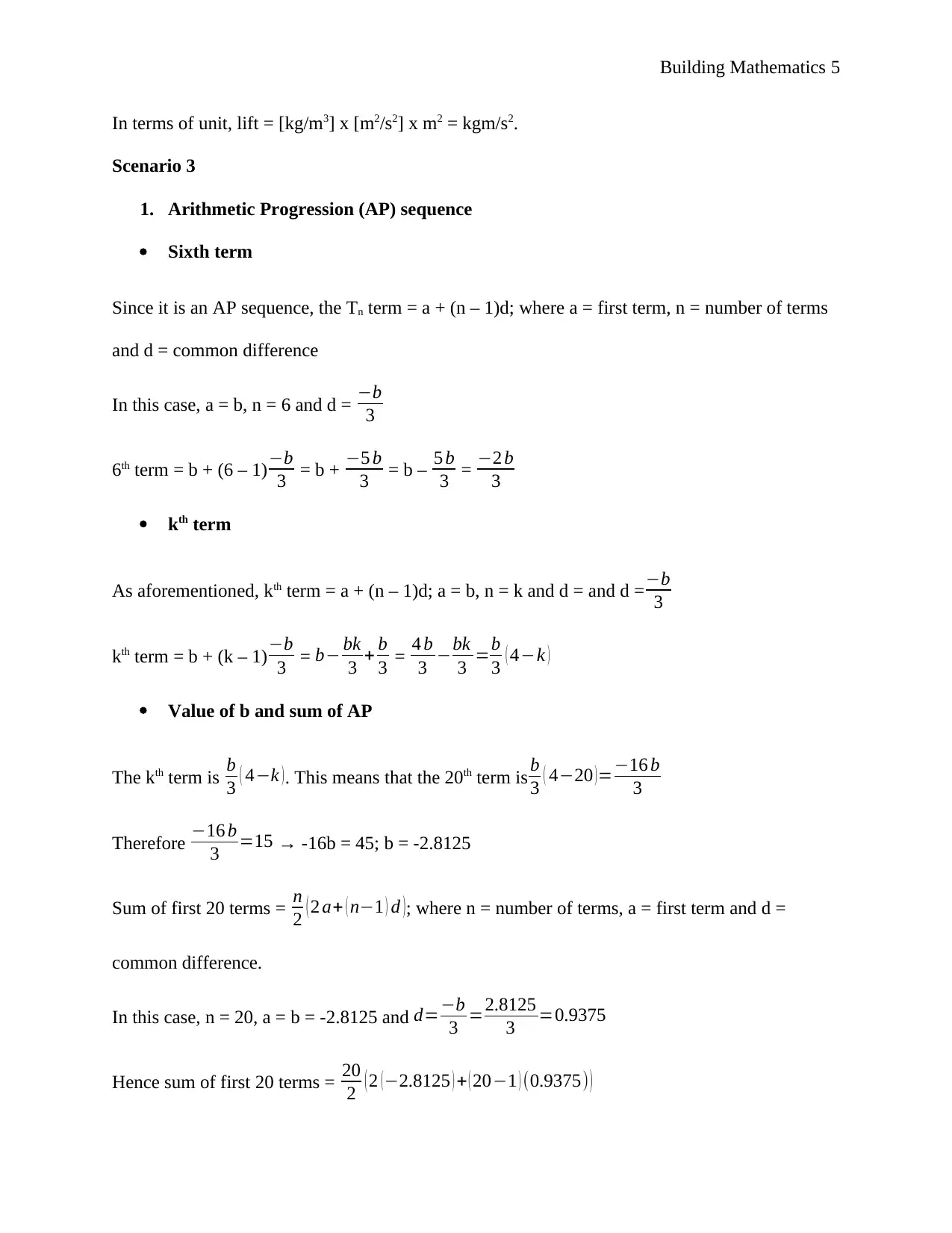
In terms of unit, lift = [kg/m3] x [m2/s2] x m2 = kgm/s2.
Scenario 3
1. Arithmetic Progression (AP) sequence
 Sixth term
Since it is an AP sequence, the Tn term = a + (n – 1)d; where a = first term, n = number of terms
and d = common difference
In this case, a = b, n = 6 and d = −b
3
6th term = b + (6 – 1) −b
3 = b + −5 b
3 = b – 5 b
3 = −2 b
3
 kth term
As aforementioned, kth term = a + (n – 1)d; a = b, n = k and d = and d =−b
3
kth term = b + (k – 1) −b
3 = b− bk
3 + b
3 = 4 b
3 −bk
3 =b
3 ( 4−k )
 Value of b and sum of AP
The kth term is b
3 ( 4−k ). This means that the 20th term is b
3 ( 4−20 )=−16 b
3
Therefore −16 b
3 =15 → -16b = 45; b = -2.8125
Sum of first 20 terms = n
2 ( 2 a+ ( n−1 ) d ); where n = number of terms, a = first term and d =
common difference.
In this case, n = 20, a = b = -2.8125 and d=−b
3 =2.8125
3 =0.9375
Hence sum of first 20 terms = 20
2 (2 (−2.8125 ) + ( 20−1 ) (0.9375) )

Building Mathematics 6
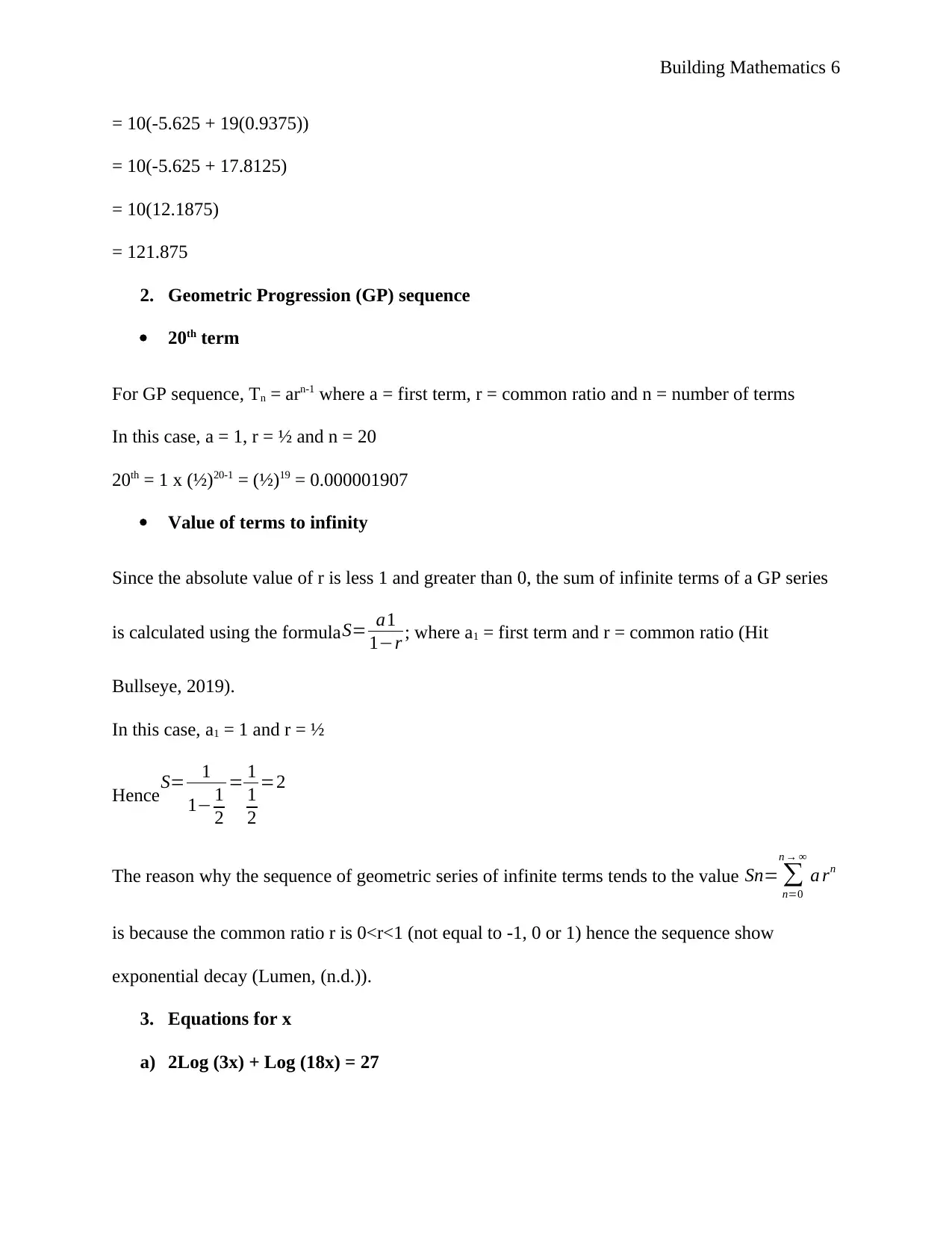
= 10(-5.625 + 19(0.9375))
= 10(-5.625 + 17.8125)
= 10(12.1875)
= 121.875
2. Geometric Progression (GP) sequence
 20th term
For GP sequence, Tn = arn-1 where a = first term, r = common ratio and n = number of terms
In this case, a = 1, r = ½ and n = 20
20th = 1 x (½)20-1 = (½)19 = 0.000001907
 Value of terms to infinity
Since the absolute value of r is less 1 and greater than 0, the sum of infinite terms of a GP series
is calculated using the formula S= a1
1−r ; where a1 = first term and r = common ratio (Hit
Bullseye, 2019).
In this case, a1 = 1 and r = ½
HenceS= 1
1− 1
2
= 1
1
2
=2
The reason why the sequence of geometric series of infinite terms tends to the value Sn= ∑
n=0
n → ∞
a rn
is because the common ratio r is 0<r<1 (not equal to -1, 0 or 1) hence the sequence show
exponential decay (Lumen, (n.d.)).
3. Equations for x
a) 2Log (3x) + Log (18x) = 27

Building Mathematics 7
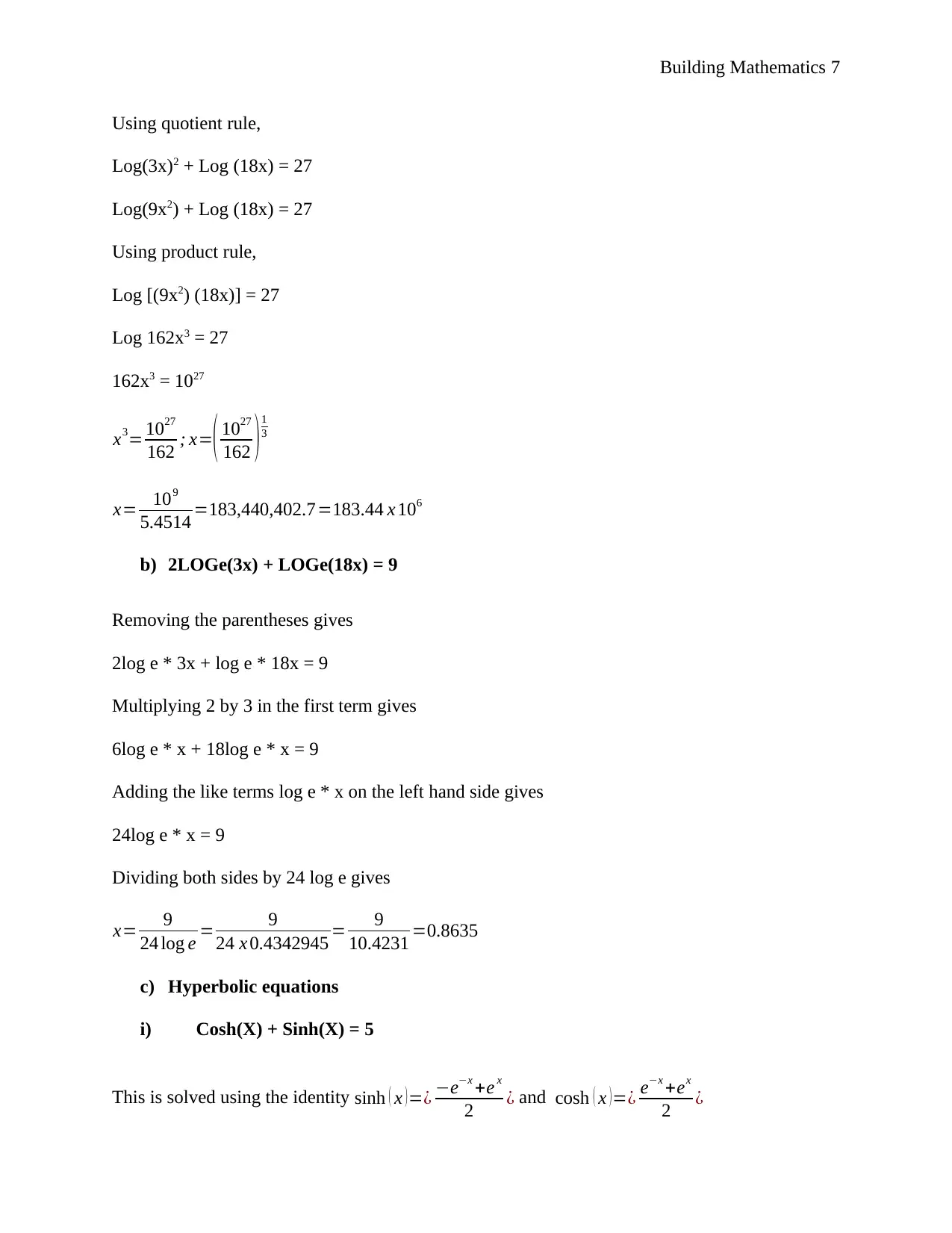
Using quotient rule,
Log(3x)2 + Log (18x) = 27
Log(9x2) + Log (18x) = 27
Using product rule,
Log [(9x2) (18x)] = 27
Log 162x3 = 27
162x3 = 1027
x3= 1027
162 ; x=( 1027
162 )1
3
x= 109
5.4514 =183,440,402.7=183.44 x 106
b) 2LOGe(3x) + LOGe(18x) = 9
Removing the parentheses gives
2log e * 3x + log e * 18x = 9
Multiplying 2 by 3 in the first term gives
6log e * x + 18log e * x = 9
Adding the like terms log e * x on the left hand side gives
24log e * x = 9
Dividing both sides by 24 log e gives
x= 9
24 log e = 9
24 x 0.4342945 = 9
10.4231 =0.8635
c) Hyperbolic equations
i) Cosh(X) + Sinh(X) = 5
This is solved using the identity sinh ( x )=¿ −e−x +e x
2 ¿ and cosh ( x )=¿ e−x +ex
2 ¿

Building Mathematics 8
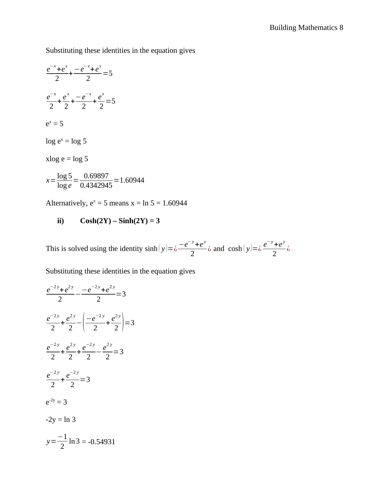
Substituting these identities in the equation gives
e−x +ex
2 + −e−x+ ex
2 =5
e−x
2 + e x
2 +−e−x
2 + ex
2 =5
ex = 5
log ex = log 5
xlog e = log 5
x= log 5
log e = 0.69897
0.4342945 =1.60944
Alternatively, ex = 5 means x = ln 5 = 1.60944
ii) Cosh(2Y) – Sinh(2Y) = 3
This is solved using the identity sinh ( y )=¿ −e− y +e y
2 ¿ and cosh ( y )=¿ e− y +e y
2 ¿
Substituting these identities in the equation gives
e−2 y+ e2 y
2 −−e−2 y +e2 y
2 =3
e−2 y
2 + e2 y
2 − (−e−2 y
2 + e2 y
2 )=3
e−2 y
2 + e2 y
2 + e−2 y
2 − e2 y
2 =3
e−2 y
2 + e−2 y
2 =3
e-2y = 3
-2y = ln 3
y=−1
2 ln 3 = -0.54931

Building Mathematics 9
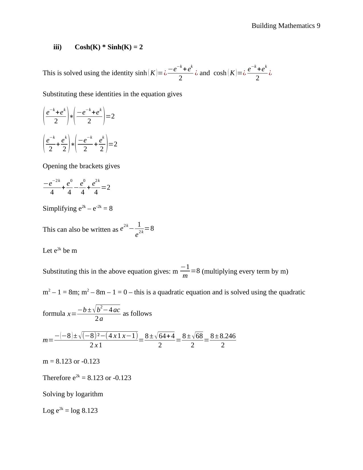
iii) Cosh(K) * Sinh(K) = 2
This is solved using the identity sinh ( K )=¿ −e−k + ek
2 ¿ and cosh ( K )=¿ e−k +ek
2 ¿
Substituting these identities in the equation gives
( e−k +ek
2 )∗(−e−k +ek
2 )=2
( e−k
2 + ek
2 )∗( −e−k
2 + ek
2 )=2
Opening the brackets gives
−e−2 k
4 + e0
4 − e0
4 + e2 k
4 =2
Simplifying e2k – e-2k = 8
This can also be written as e2 k− 1
e2 k =8
Let e2k be m
Substituting this in the above equation gives: m −1
m =8 (multiplying every term by m)
m2 – 1 = 8m; m2 – 8m – 1 = 0 – this is a quadratic equation and is solved using the quadratic
formula x=−b ± √ b2−4 ac
2 a as follows
m=− (−8 ) ± √(−8)²−(4 x 1 x−1)
2 x 1 = 8 ± √ 64+ 4
2 = 8 ± √68
2 = 8 ± 8.246
2
m = 8.123 or -0.123
Therefore e2k = 8.123 or -0.123
Solving by logarithm
Log e2k = log 8.123

Building Mathematics 10
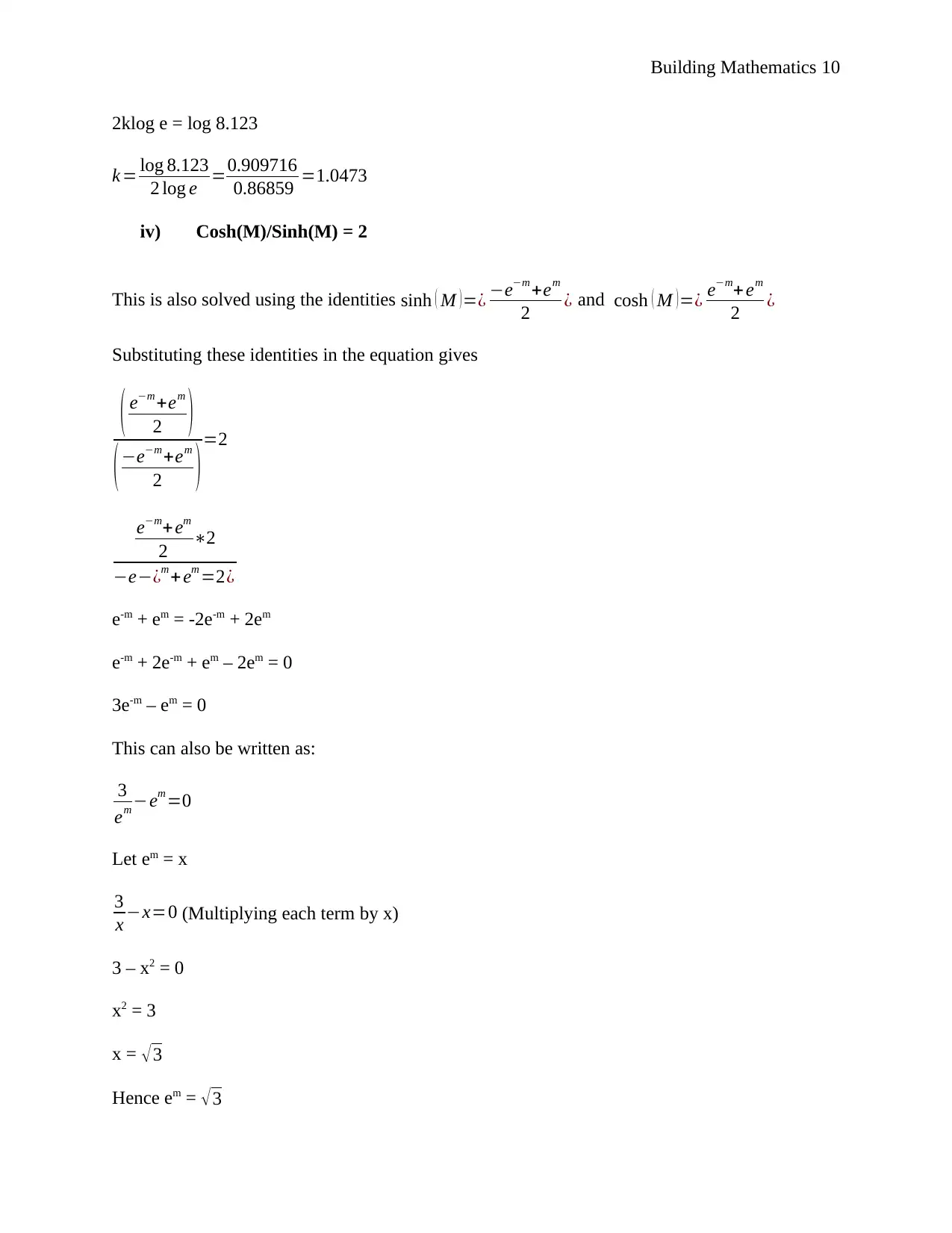
2klog e = log 8.123
k = log 8.123
2 log e =0.909716
0.86859 =1.0473
iv) Cosh(M)/Sinh(M) = 2
This is also solved using the identities sinh ( M ) =¿ −e−m +em
2 ¿ and cosh ( M )=¿ e−m+ em
2 ¿
Substituting these identities in the equation gives
( e−m +em
2 )
(−e−m +em
2 )=2
e−m+ em
2 ∗2
−e−¿m + em =2¿
e-m + em = -2e-m + 2em
e-m + 2e-m + em – 2em = 0
3e-m – em = 0
This can also be written as:
3
em −em =0
Let em = x
3
x −x=0 (Multiplying each term by x)
3 – x2 = 0
x2 = 3
x = √3
Hence em = √3

Building Mathematics 11
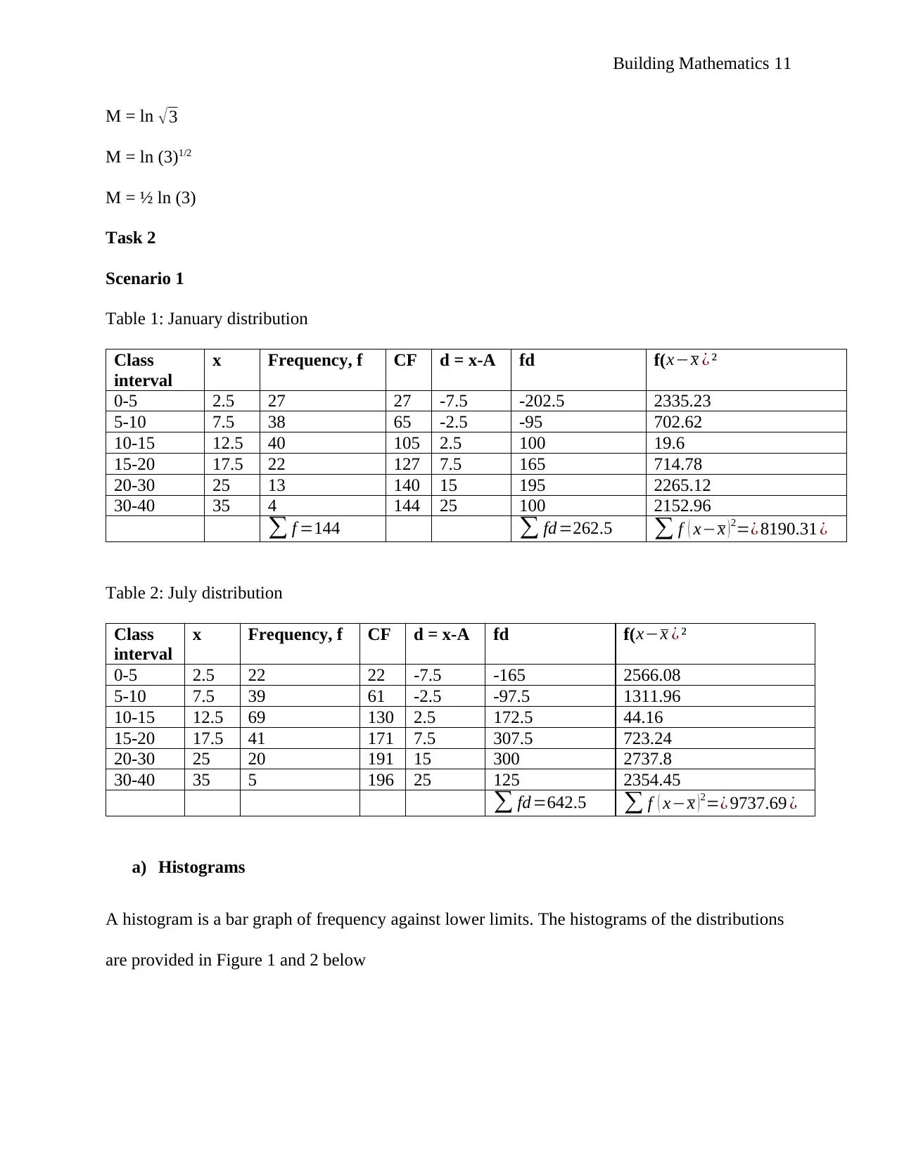
M = ln √3
M = ln (3)1/2
M = ½ ln (3)
Task 2
Scenario 1
Table 1: January distribution
Class
interval
x Frequency, f CF d = x-A fd f(x−x ¿ ²
0-5 2.5 27 27 -7.5 -202.5 2335.23
5-10 7.5 38 65 -2.5 -95 702.62
10-15 12.5 40 105 2.5 100 19.6
15-20 17.5 22 127 7.5 165 714.78
20-30 25 13 140 15 195 2265.12
30-40 35 4 144 25 100 2152.96
∑ f =144 ∑ fd =262.5 ∑ f ( x−x )2=¿ 8190.31 ¿
Table 2: July distribution
Class
interval
x Frequency, f CF d = x-A fd f( x−x ¿ ²
0-5 2.5 22 22 -7.5 -165 2566.08
5-10 7.5 39 61 -2.5 -97.5 1311.96
10-15 12.5 69 130 2.5 172.5 44.16
15-20 17.5 41 171 7.5 307.5 723.24
20-30 25 20 191 15 300 2737.8
30-40 35 5 196 25 125 2354.45
∑ fd=642.5 ∑ f ( x−x ) 2=¿ 9737.69 ¿
a) Histograms
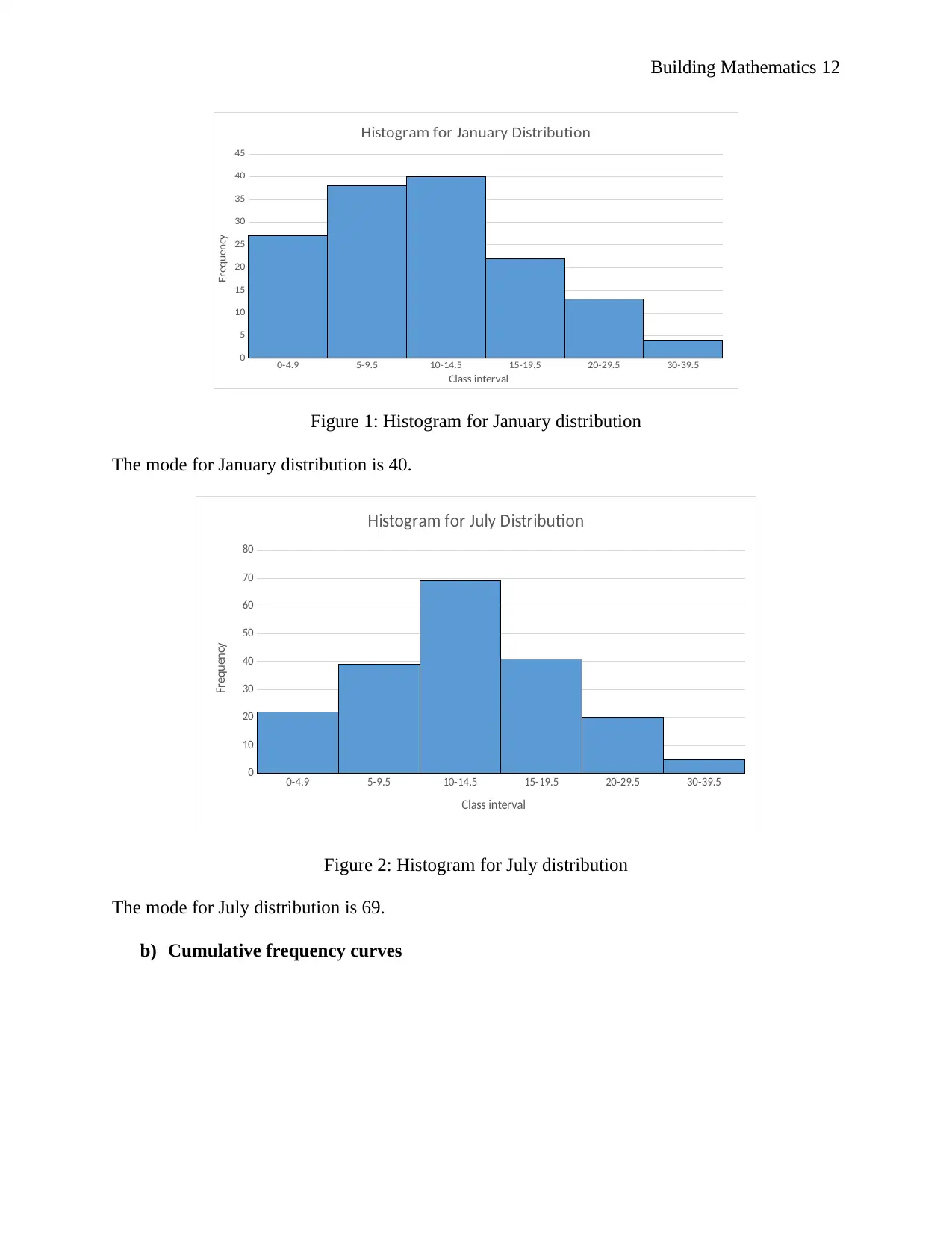
A histogram is a bar graph of frequency against lower limits. The histograms of the distributions
are provided in Figure 1 and 2 below

Building Mathematics 12
0-4.9 5-9.5 10-14.5 15-19.5 20-29.5 30-39.5
0
5
10
15
20
25
30
35
40
45
Histogram for January Distribution
Class interval
Frequency
Figure 1: Histogram for January distribution
The mode for January distribution is 40.
0-4.9 5-9.5 10-14.5 15-19.5 20-29.5 30-39.5
0
10
20
30
40
50
60
70
80
Histogram for July Distribution
Class interval
Frequency
Figure 2: Histogram for July distribution
The mode for July distribution is 69.
b) Cumulative frequency curves

Building Mathematics 13
0 5 10 15 20 25 30 35 40 45
0
20
40
60
80
100
120
140
160
Cumulative Frequency Curve for January Distribution
Class Interval
Cumulative Frequency
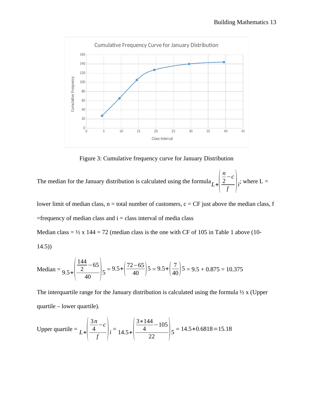
Figure 3: Cumulative frequency curve for January Distribution
The median for the January distribution is calculated using the formulaL+( n
2 −c
f )i; where L =
lower limit of median class, n = total number of customers, c = CF just above the median class, f
=frequency of median class and i = class interval of media class
Median class = ½ x 144 = 72 (median class is the one with CF of 105 in Table 1 above (10-
14.5))
Median = 9.5+ ( 144
2 −65
40 ) 5 = 9.5+ ( 72−65
40 )5 = 9.5+ ( 7
40 )5 = 9.5 + 0.875 = 10.375
The interquartile range for the January distribution is calculated using the formula ½ x (Upper
quartile – lower quartile).
Upper quartile = L+( 3 n
4 −c
f )i = 14.5+ ( 3∗144
4 −105
22 )5 = 14.5+0.6818=15.18

Building Mathematics 14
Lower quartile = L+( n
4 −c
f ) i = 4.5+ ( 1∗144
4 −27
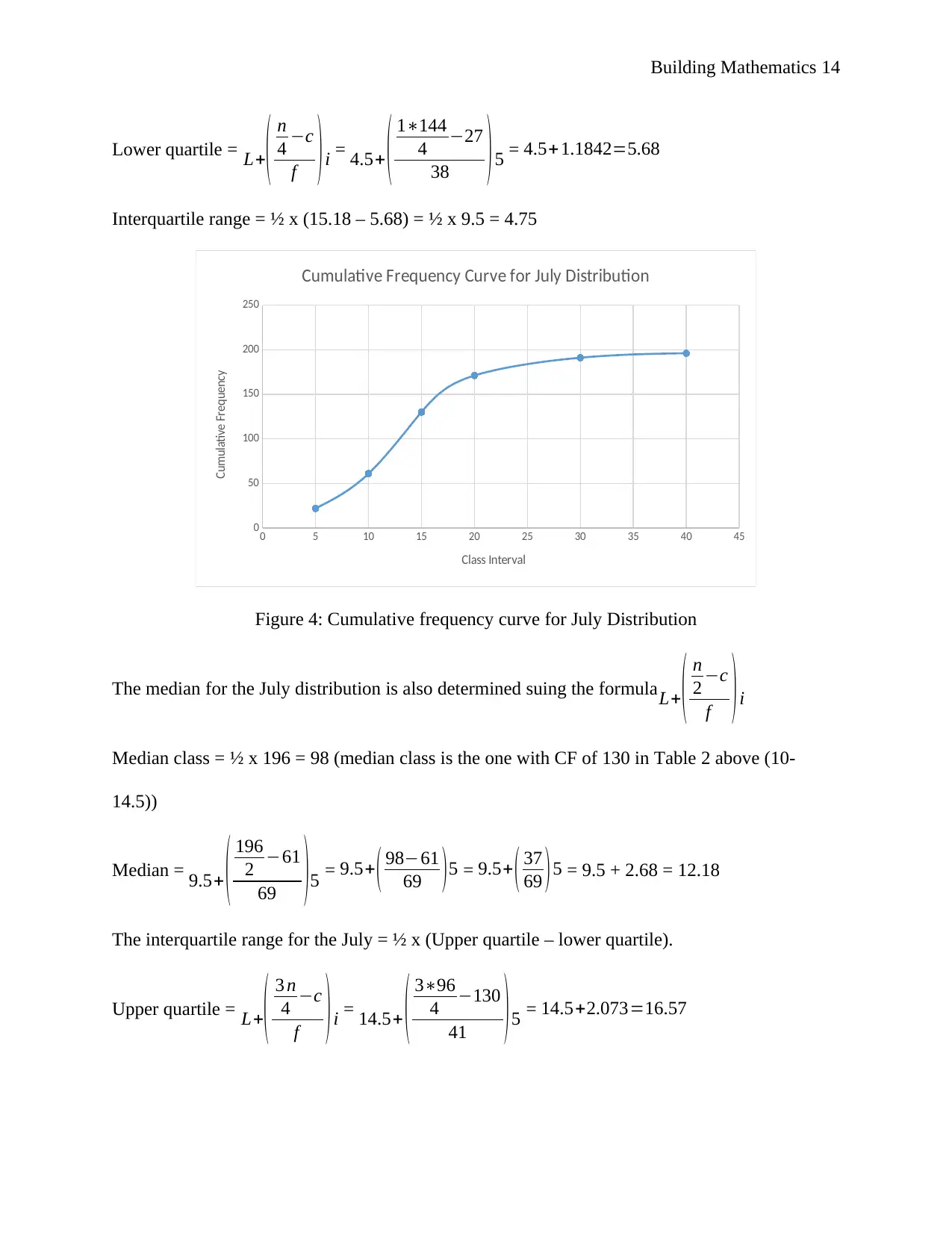
38 )5 = 4.5+1.1842=5.68
Interquartile range = ½ x (15.18 – 5.68) = ½ x 9.5 = 4.75
0 5 10 15 20 25 30 35 40 45
0
50
100
150
200
250
Cumulative Frequency Curve for July Distribution
Class Interval
Cumulative Frequency
Figure 4: Cumulative frequency curve for July Distribution
The median for the July distribution is also determined suing the formula L+( n
2 −c
f ) i
Median class = ½ x 196 = 98 (median class is the one with CF of 130 in Table 2 above (10-
14.5))
Median = 9.5+ ( 196
2 −61
69 )5 = 9.5+ ( 98−61
69 )5 = 9.5+ ( 37
69 )5 = 9.5 + 2.68 = 12.18
The interquartile range for the July = ½ x (Upper quartile – lower quartile).
Upper quartile = L+( 3 n
4 −c
f ) i = 14.5+ ( 3∗96
4 −130
41 ) 5 = 14.5+2.073=16.57

Building Mathematics 15
Lower quartile = L+( n
4 −c
f ) i = 4.5+ ( 1∗196
4 −22
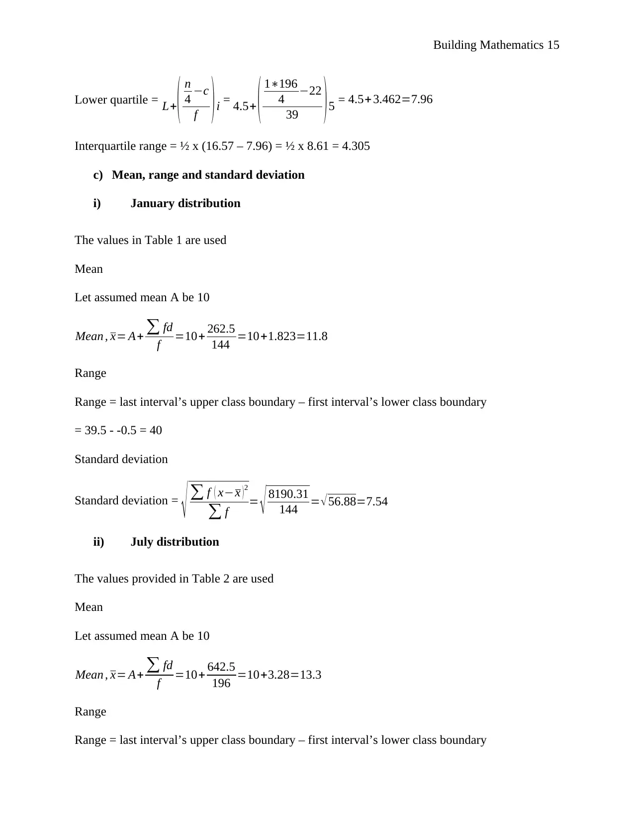
39 ) 5 = 4.5+ 3.462=7.96
Interquartile range = ½ x (16.57 – 7.96) = ½ x 8.61 = 4.305
c) Mean, range and standard deviation
i) January distribution
The values in Table 1 are used
Mean
Let assumed mean A be 10
Mean , x= A+ ∑ fd
f =10+ 262.5
144 =10+1.823=11.8
Range
Range = last interval’s upper class boundary – first interval’s lower class boundary
= 39.5 - -0.5 = 40
Standard deviation
Standard deviation =
√ ∑ f ( x−x )2
∑ f = √ 8190.31
144 = √ 56.88=7.54
ii) July distribution
The values provided in Table 2 are used
Mean
Let assumed mean A be 10
Mean , x= A+ ∑ fd
f =10+ 642.5
196 =10+3.28=13.3
Range
Range = last interval’s upper class boundary – first interval’s lower class boundary

Building Mathematics 16
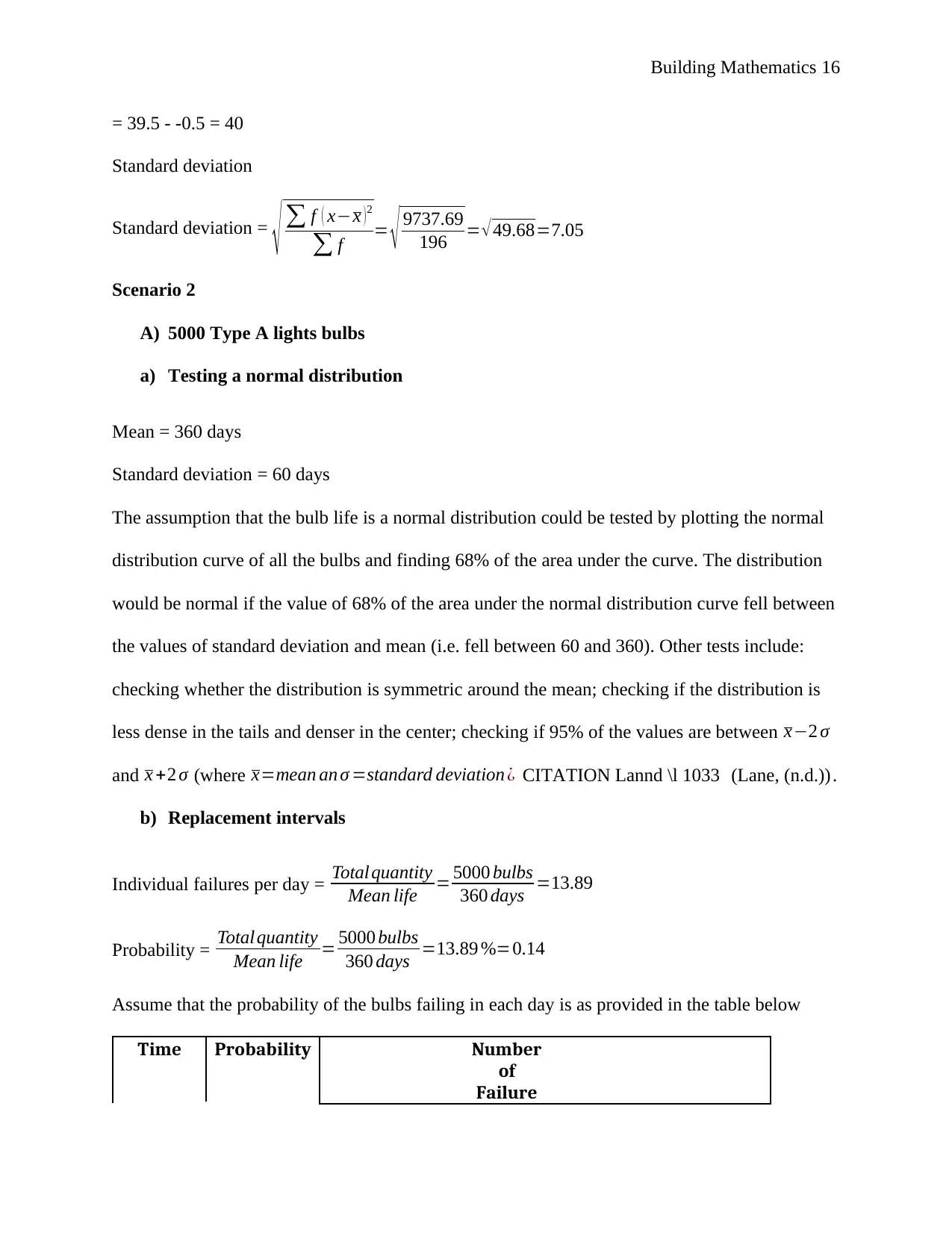
= 39.5 - -0.5 = 40
Standard deviation
Standard deviation =
√ ∑ f ( x−x )2
∑ f = √ 9737.69
196 = √ 49.68=7.05
Scenario 2
A) 5000 Type A lights bulbs
a) Testing a normal distribution
Mean = 360 days
Standard deviation = 60 days
The assumption that the bulb life is a normal distribution could be tested by plotting the normal
distribution curve of all the bulbs and finding 68% of the area under the curve. The distribution
would be normal if the value of 68% of the area under the normal distribution curve fell between
the values of standard deviation and mean (i.e. fell between 60 and 360). Other tests include:
checking whether the distribution is symmetric around the mean; checking if the distribution is
less dense in the tails and denser in the center; checking if 95% of the values are between x−2 σ
and x +2 σ (where x=mean an σ =standard deviation ¿ CITATION Lannd \l 1033 (Lane, (n.d.)).
b) Replacement intervals
Individual failures per day = Total quantity
Mean life = 5000 bulbs
360 days =13.89
Probability = Total quantity
Mean life = 5000 bulbs
360 days =13.89 %=0.14
Assume that the probability of the bulbs failing in each day is as provided in the table below
Time Probability Number
of
Failure

Building Mathematics 17
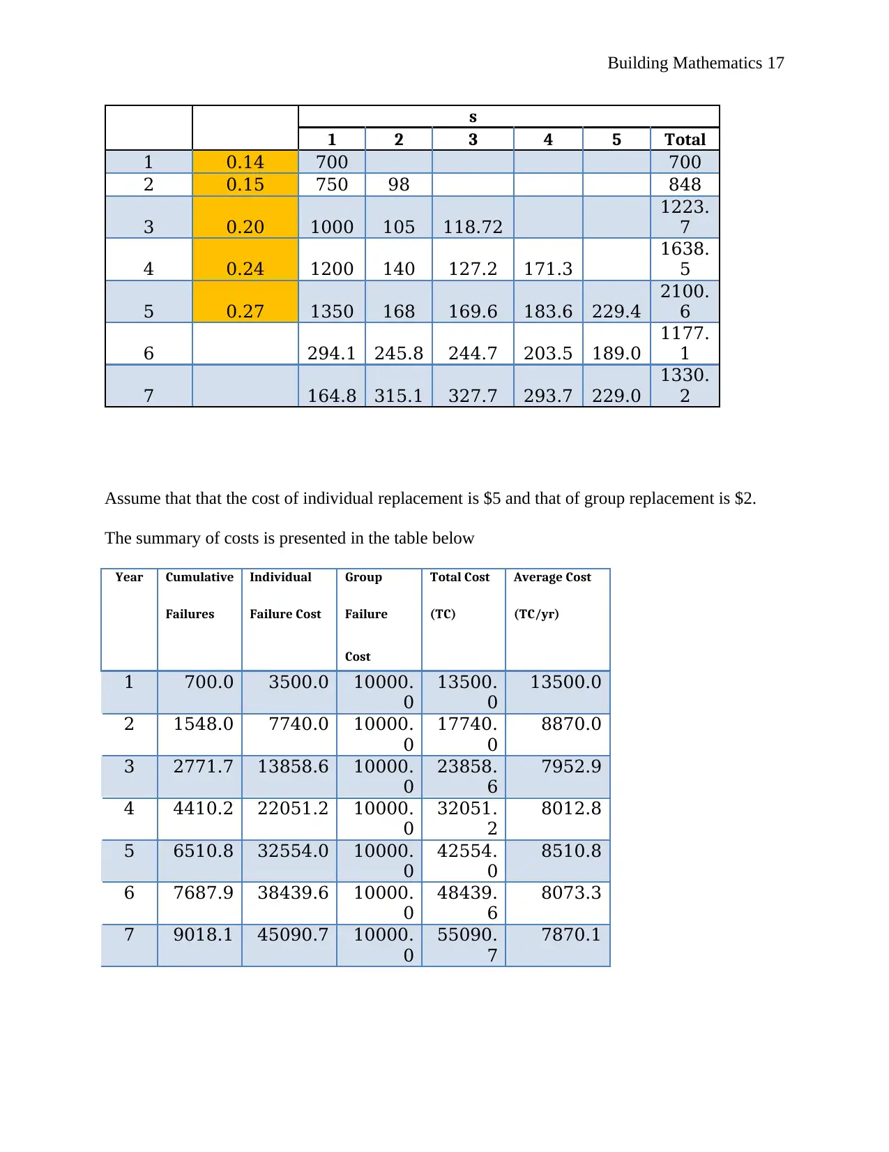
s
1 2 3 4 5 Total
1 0.14 700 700
2 0.15 750 98 848
3 0.20 1000 105 118.72
1223.
7
4 0.24 1200 140 127.2 171.3
1638.
5
5 0.27 1350 168 169.6 183.6 229.4
2100.
6
6 294.1 245.8 244.7 203.5 189.0
1177.
1
7 164.8 315.1 327.7 293.7 229.0
1330.
2
Assume that that the cost of individual replacement is $5 and that of group replacement is $2.
The summary of costs is presented in the table below
Year Cumulative Individual Group Total Cost Average Cost
Failures Failure Cost Failure (TC) (TC/yr)
Cost
1 700.0 3500.0 10000.
0
13500.
0
13500.0
2 1548.0 7740.0 10000.
0
17740.
0
8870.0
3 2771.7 13858.6 10000.
0
23858.
6
7952.9
4 4410.2 22051.2 10000.
0
32051.
2
8012.8
5 6510.8 32554.0 10000.
0
42554.
0
8510.8
6 7687.9 38439.6 10000.
0
48439.
6
8073.3
7 9018.1 45090.7 10000.
0
55090.
7
7870.1

Building Mathematics 18
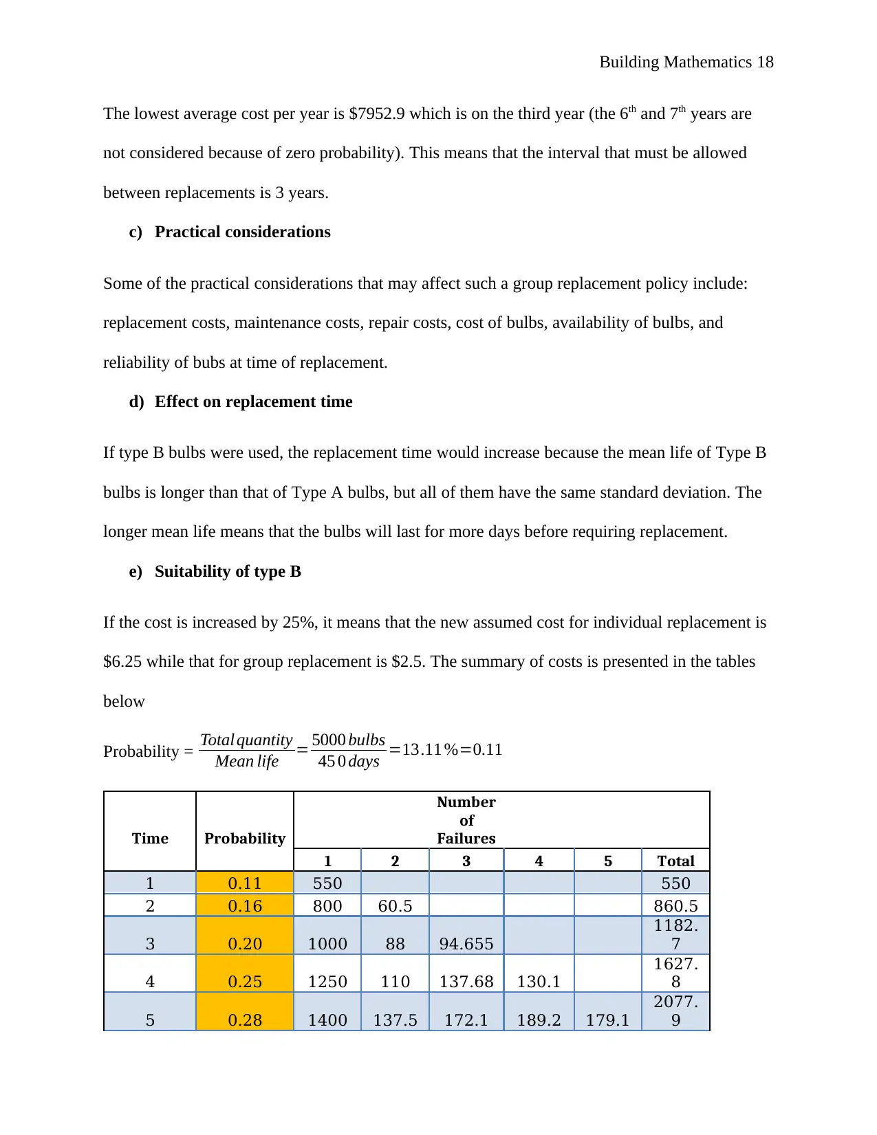
The lowest average cost per year is $7952.9 which is on the third year (the 6th and 7th years are
not considered because of zero probability). This means that the interval that must be allowed
between replacements is 3 years.
c) Practical considerations
Some of the practical considerations that may affect such a group replacement policy include:
replacement costs, maintenance costs, repair costs, cost of bulbs, availability of bulbs, and
reliability of bubs at time of replacement.
d) Effect on replacement time
If type B bulbs were used, the replacement time would increase because the mean life of Type B
bulbs is longer than that of Type A bulbs, but all of them have the same standard deviation. The
longer mean life means that the bulbs will last for more days before requiring replacement.
e) Suitability of type B
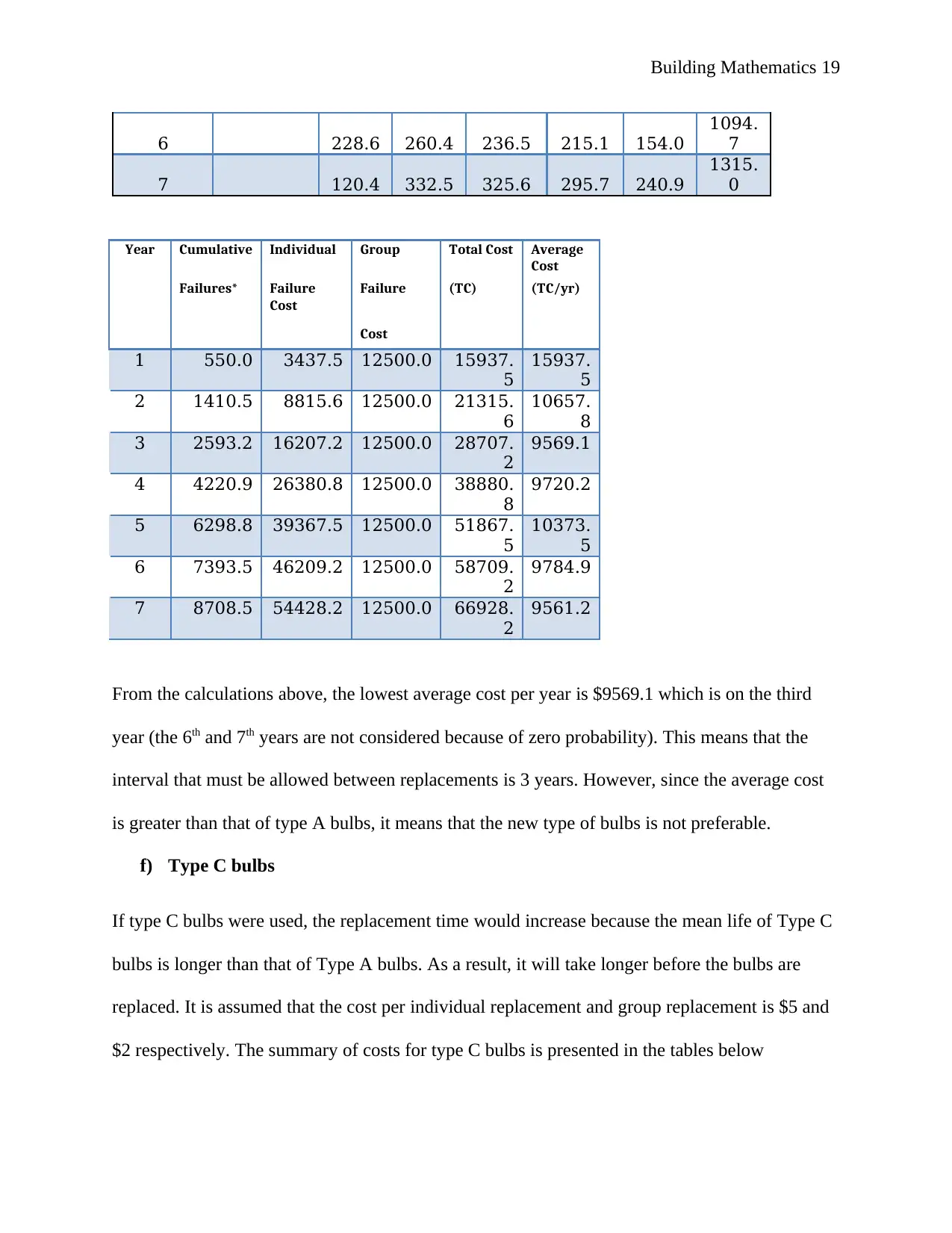
If the cost is increased by 25%, it means that the new assumed cost for individual replacement is
$6.25 while that for group replacement is $2.5. The summary of costs is presented in the tables
below
Probability = Total quantity
Mean life = 5000 bulbs
45 0 days =13.11 %=0.11
Time Probability
Number
of
Failures
1 2 3 4 5 Total
1 0.11 550 550
2 0.16 800 60.5 860.5
3 0.20 1000 88 94.655
1182.
7
4 0.25 1250 110 137.68 130.1
1627.
8
5 0.28 1400 137.5 172.1 189.2 179.1
2077.
9

Building Mathematics 19
6 228.6 260.4 236.5 215.1 154.0
1094.
7
7 120.4 332.5 325.6 295.7 240.9
1315.
0
Year Cumulative Individual Group Total Cost Average
Cost
Failures* Failure
Cost
Failure (TC) (TC/yr)
Cost
1 550.0 3437.5 12500.0 15937.
5
15937.
5
2 1410.5 8815.6 12500.0 21315.
6
10657.
8
3 2593.2 16207.2 12500.0 28707.
2
9569.1
4 4220.9 26380.8 12500.0 38880.
8
9720.2
5 6298.8 39367.5 12500.0 51867.
5
10373.
5
6 7393.5 46209.2 12500.0 58709.
2
9784.9
7 8708.5 54428.2 12500.0 66928.
2
9561.2
From the calculations above, the lowest average cost per year is $9569.1 which is on the third
year (the 6th and 7th years are not considered because of zero probability). This means that the
interval that must be allowed between replacements is 3 years. However, since the average cost
is greater than that of type A bulbs, it means that the new type of bulbs is not preferable.
f) Type C bulbs
If type C bulbs were used, the replacement time would increase because the mean life of Type C
bulbs is longer than that of Type A bulbs. As a result, it will take longer before the bulbs are
replaced. It is assumed that the cost per individual replacement and group replacement is $5 and
$2 respectively. The summary of costs for type C bulbs is presented in the tables below

Building Mathematics 20
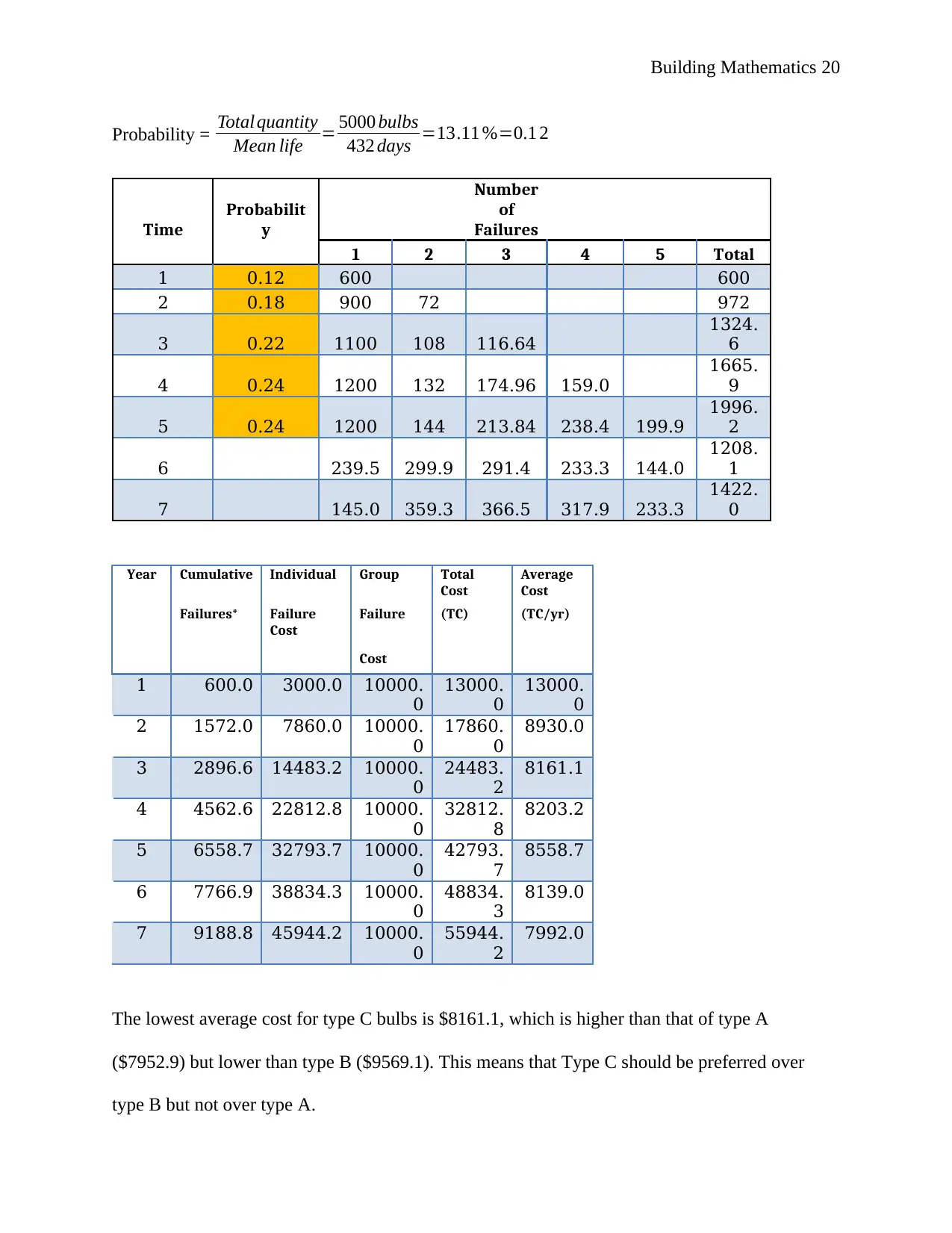
Probability = Total quantity
Mean life = 5000 bulbs
432 days =13.11 %=0.1 2
Time
Probabilit
y
Number
of
Failures
1 2 3 4 5 Total
1 0.12 600 600
2 0.18 900 72 972
3 0.22 1100 108 116.64
1324.
6
4 0.24 1200 132 174.96 159.0
1665.
9
5 0.24 1200 144 213.84 238.4 199.9
1996.
2
6 239.5 299.9 291.4 233.3 144.0
1208.
1
7 145.0 359.3 366.5 317.9 233.3
1422.
0
Year Cumulative Individual Group Total
Cost
Average
Cost
Failures* Failure
Cost
Failure (TC) (TC/yr)
Cost
1 600.0 3000.0 10000.
0
13000.
0
13000.
0
2 1572.0 7860.0 10000.
0
17860.
0
8930.0
3 2896.6 14483.2 10000.
0
24483.
2
8161.1
4 4562.6 22812.8 10000.
0
32812.
8
8203.2
5 6558.7 32793.7 10000.
0
42793.
7
8558.7
6 7766.9 38834.3 10000.
0
48834.
3
8139.0
7 9188.8 45944.2 10000.
0
55944.
2
7992.0
The lowest average cost for type C bulbs is $8161.1, which is higher than that of type A
($7952.9) but lower than type B ($9569.1). This means that Type C should be preferred over
type B but not over type A.

Building Mathematics 21
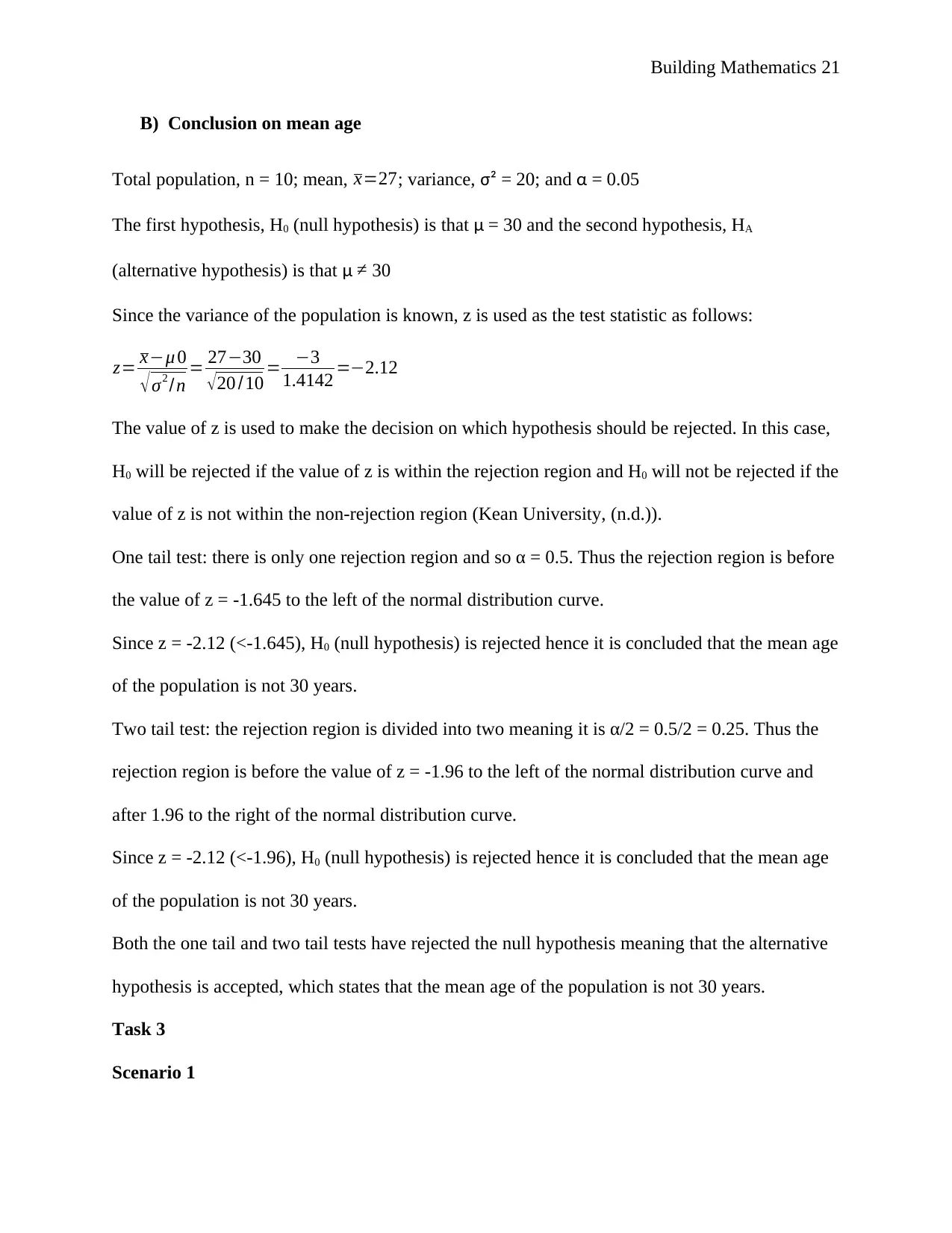
B) Conclusion on mean age
Total population, n = 10; mean, x=27; variance, σ² = 20; and α = 0.05
The first hypothesis, H0 (null hypothesis) is that μ = 30 and the second hypothesis, HA
(alternative hypothesis) is that μ ≠ 30
Since the variance of the population is known, z is used as the test statistic as follows:
z= x−μ 0
√ σ2 /n = 27−30
√ 20 /10 = −3
1.4142 =−2.12
The value of z is used to make the decision on which hypothesis should be rejected. In this case,
H0 will be rejected if the value of z is within the rejection region and H0 will not be rejected if the
value of z is not within the non-rejection region (Kean University, (n.d.)).
One tail test: there is only one rejection region and so α = 0.5. Thus the rejection region is before
the value of z = -1.645 to the left of the normal distribution curve.
Since z = -2.12 (<-1.645), H0 (null hypothesis) is rejected hence it is concluded that the mean age
of the population is not 30 years.
Two tail test: the rejection region is divided into two meaning it is α/2 = 0.5/2 = 0.25. Thus the
rejection region is before the value of z = -1.96 to the left of the normal distribution curve and
after 1.96 to the right of the normal distribution curve.
Since z = -2.12 (<-1.96), H0 (null hypothesis) is rejected hence it is concluded that the mean age
of the population is not 30 years.
Both the one tail and two tail tests have rejected the null hypothesis meaning that the alternative
hypothesis is accepted, which states that the mean age of the population is not 30 years.
Task 3
Scenario 1

Building Mathematics 22
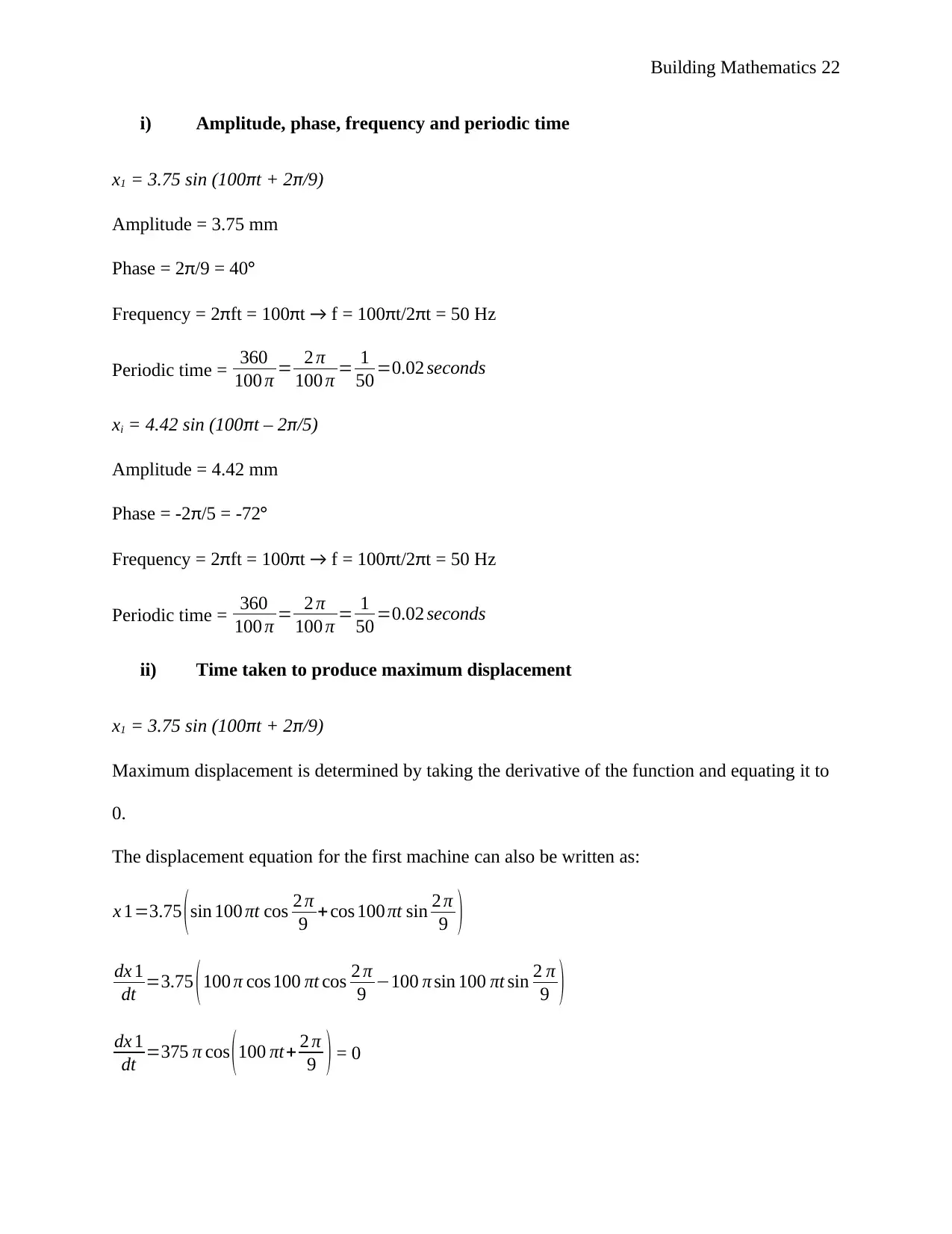
i) Amplitude, phase, frequency and periodic time
x1 = 3.75 sin (100πt + 2π/9)
Amplitude = 3.75 mm
Phase = 2π/9 = 40°
Frequency = 2πft = 100πt → f = 100πt/2πt = 50 Hz
Periodic time = 360
100 π = 2 π
100 π = 1
50 =0.02 seconds
xi = 4.42 sin (100πt – 2π/5)
Amplitude = 4.42 mm
Phase = -2π/5 = -72°
Frequency = 2πft = 100πt → f = 100πt/2πt = 50 Hz
Periodic time = 360
100 π = 2 π
100 π = 1
50 =0.02 seconds
ii) Time taken to produce maximum displacement
x1 = 3.75 sin (100πt + 2π/9)
Maximum displacement is determined by taking the derivative of the function and equating it to
0.
The displacement equation for the first machine can also be written as:
x 1=3.75 ( sin 100 πt cos 2 π
9 +cos 100 πt sin 2 π
9 )
dx 1
dt =3.75 (100 π cos 100 πt cos 2 π
9 −100 π sin 100 πt sin 2 π
9 )
dx 1
dt =375 π cos ( 100 πt+ 2 π
9 ) = 0

Building Mathematics 23
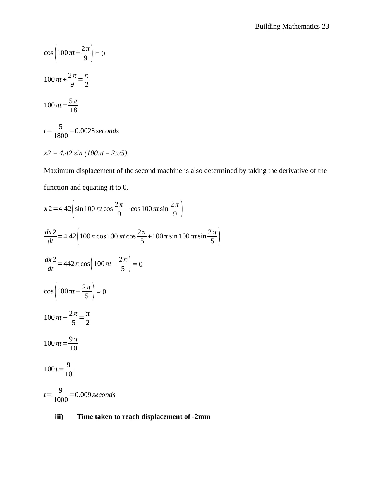
cos (100 πt + 2 π
9 ) = 0
100 πt + 2 π
9 = π
2
100 πt= 5 π
18
t= 5
1800 =0.0028 seconds
x2 = 4.42 sin (100πt – 2π/5)
Maximum displacement of the second machine is also determined by taking the derivative of the
function and equating it to 0.
x 2=4.42 (sin100 πt cos 2 π
9 −cos 100 πt sin 2 π
9 )
dx 2
dt =4.42 (100 π cos 100 πt cos 2 π
5 +100 π sin 100 πt sin 2 π
5 )
dx 2
dt =442 π cos (100 πt− 2 π
5 ) = 0
cos (100 πt − 2 π
5 ) = 0
100 πt− 2 π
5 = π
2
100 πt= 9 π
10
100 t= 9
10
t= 9
1000 =0.009 seconds
iii) Time taken to reach displacement of -2mm

Building Mathematics 24
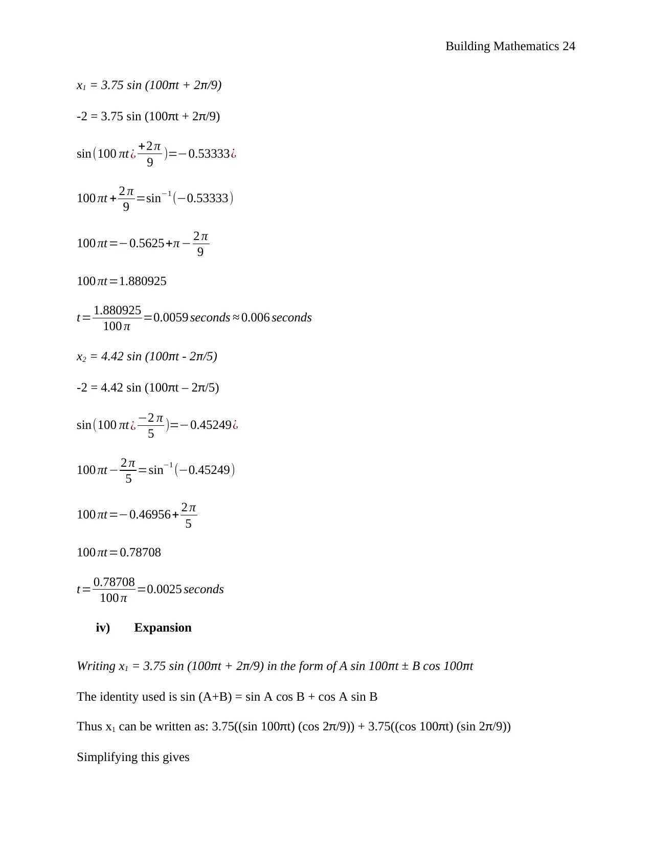
x1 = 3.75 sin (100πt + 2π/9)
-2 = 3.75 sin (100πt + 2π/9)
sin(100 πt ¿ +2 π
9 )=−0.53333¿
100 πt + 2 π
9 =sin−1 (−0.53333)
100 πt=−0.5625+π − 2 π
9
100 πt=1.880925
t= 1.880925
100 π =0.0059 seconds ≈ 0.006 seconds
x2 = 4.42 sin (100πt - 2π/5)
-2 = 4.42 sin (100πt – 2π/5)
sin(100 πt¿ −2 π
5 )=−0.45249¿
100 πt− 2 π
5 =sin−1 (−0.45249)
100 πt=−0.46956+ 2 π
5
100 πt=0.78708
t= 0.78708
100 π =0.0025 seconds
iv) Expansion
Writing x1 = 3.75 sin (100πt + 2π/9) in the form of A sin 100πt ± B cos 100πt
The identity used is sin (A+B) = sin A cos B + cos A sin B
Thus x1 can be written as: 3.75((sin 100πt) (cos 2π/9)) + 3.75((cos 100πt) (sin 2π/9))
Simplifying this gives

Building Mathematics 25
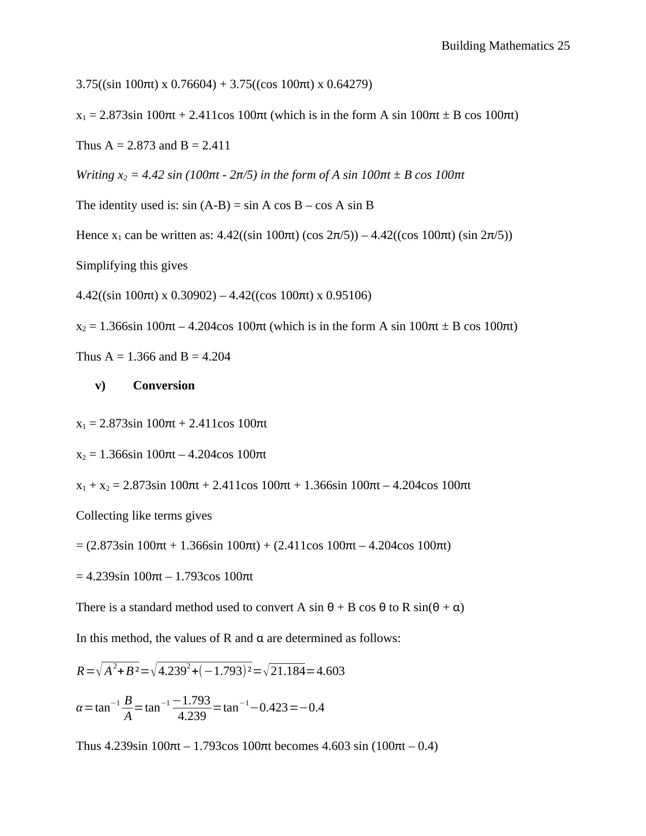
3.75((sin 100πt) x 0.76604) + 3.75((cos 100πt) x 0.64279)
x1 = 2.873sin 100πt + 2.411cos 100πt (which is in the form A sin 100πt ± B cos 100πt)
Thus A = 2.873 and B = 2.411
Writing x2 = 4.42 sin (100πt - 2π/5) in the form of A sin 100πt ± B cos 100πt
The identity used is: sin (A-B) = sin A cos B – cos A sin B
Hence x1 can be written as: 4.42((sin 100πt) (cos 2π/5)) – 4.42((cos 100πt) (sin 2π/5))
Simplifying this gives
4.42((sin 100πt) x 0.30902) – 4.42((cos 100πt) x 0.95106)
x2 = 1.366sin 100πt – 4.204cos 100πt (which is in the form A sin 100πt ± B cos 100πt)
Thus A = 1.366 and B = 4.204
v) Conversion
x1 = 2.873sin 100πt + 2.411cos 100πt
x2 = 1.366sin 100πt – 4.204cos 100πt
x1 + x2 = 2.873sin 100πt + 2.411cos 100πt + 1.366sin 100πt – 4.204cos 100πt
Collecting like terms gives
= (2.873sin 100πt + 1.366sin 100πt) + (2.411cos 100πt – 4.204cos 100πt)
= 4.239sin 100πt – 1.793cos 100πt
There is a standard method used to convert A sin θ + B cos θ to R sin(θ + α)
In this method, the values of R and α are determined as follows:
R= √ A2+ B ²= √ 4.2392 +(−1.793)²= √ 21.184=4.603
α =tan−1 B
A =tan−1 −1.793
4.239 =tan−1−0.423=−0.4
Thus 4.239sin 100πt – 1.793cos 100πt becomes 4.603 sin (100πt – 0.4)

Building Mathematics 26
vi) Table
x1 = 3.75 sin (100πt + 2π/9)
x2 = 4.42 sin (100πt - 2π/5)
x1 + x2 = 4.603 sin (100πt – 0.4)
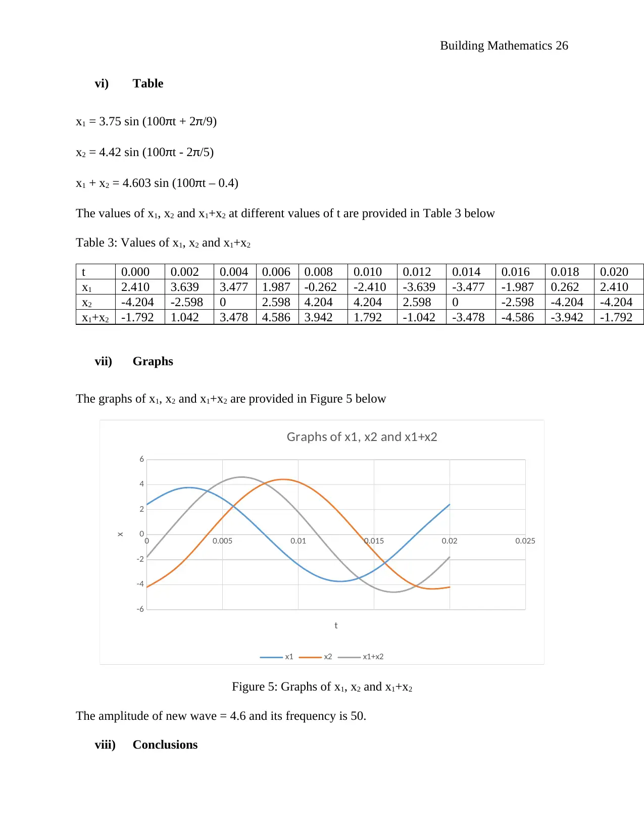
The values of x1, x2 and x1+x2 at different values of t are provided in Table 3 below
Table 3: Values of x1, x2 and x1+x2
t 0.000 0.002 0.004 0.006 0.008 0.010 0.012 0.014 0.016 0.018 0.020
x1 2.410 3.639 3.477 1.987 -0.262 -2.410 -3.639 -3.477 -1.987 0.262 2.410
x2 -4.204 -2.598 0 2.598 4.204 4.204 2.598 0 -2.598 -4.204 -4.204
x1+x2 -1.792 1.042 3.478 4.586 3.942 1.792 -1.042 -3.478 -4.586 -3.942 -1.792
vii) Graphs
The graphs of x1, x2 and x1+x2 are provided in Figure 5 below
0 0.005 0.01 0.015 0.02 0.025
-6
-4
-2
0
2
4
6
Graphs of x1, x2 and x1+x2
x1 x2 x1+x2
t
x
Figure 5: Graphs of x1, x2 and x1+x2
The amplitude of new wave = 4.6 and its frequency is 50.
viii) Conclusions

Building Mathematics 27
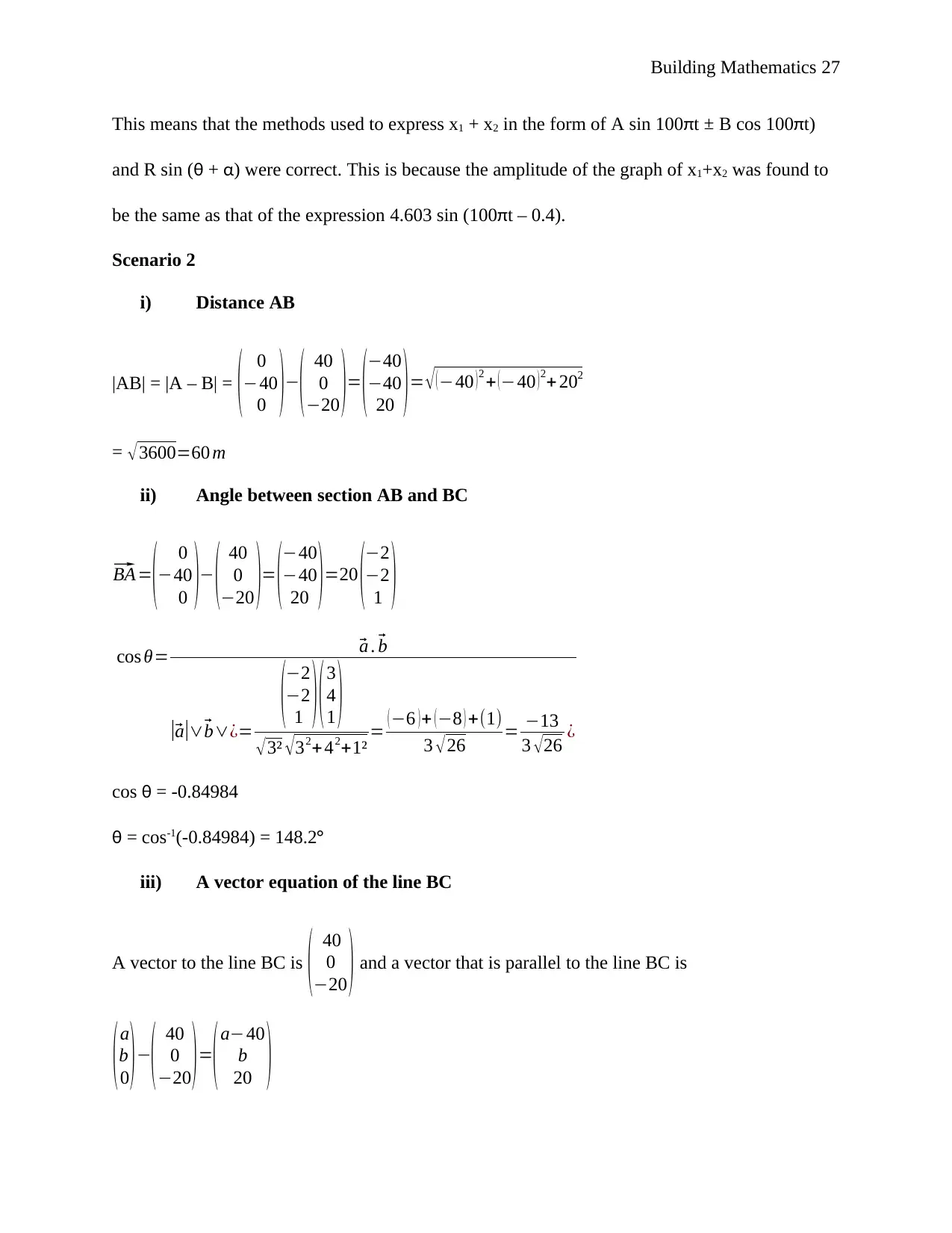
This means that the methods used to express x1 + x2 in the form of A sin 100πt ± B cos 100πt)
and R sin (θ + α) were correct. This is because the amplitude of the graph of x1+x2 was found to
be the same as that of the expression 4.603 sin (100πt – 0.4).
Scenario 2
i) Distance AB
|AB| = |A – B| = ( 0
−40
0 )−
( 40
0
−20 )= (
−40
−40
20 ) = √ ( −40 ) 2 + ( −40 ) 2+ 202
= √3600=60 m
ii) Angle between section AB and BC⃗
BA=
(−
0
40
0 )− ( 40
0
−20 )= (−40
−40
20 )=20 (−2
−2
1 )
cos θ=⃗ a .⃗ b
|⃗a|∨⃗ b∨¿=
(−2
−2
1 )(3
4
1 )
√3² √32+42+1² = (−6 )+ (−8 ) +(1)
3 √26 = −13
3 √26 ¿
cos θ = -0.84984
θ = cos-1(-0.84984) = 148.2°
iii) A vector equation of the line BC
A vector to the line BC is ( 40
0
−20 ) and a vector that is parallel to the line BC is
(a
b
0 )−
( 40
0
−20)=
(a−40
b
20 )

Building Mathematics 28
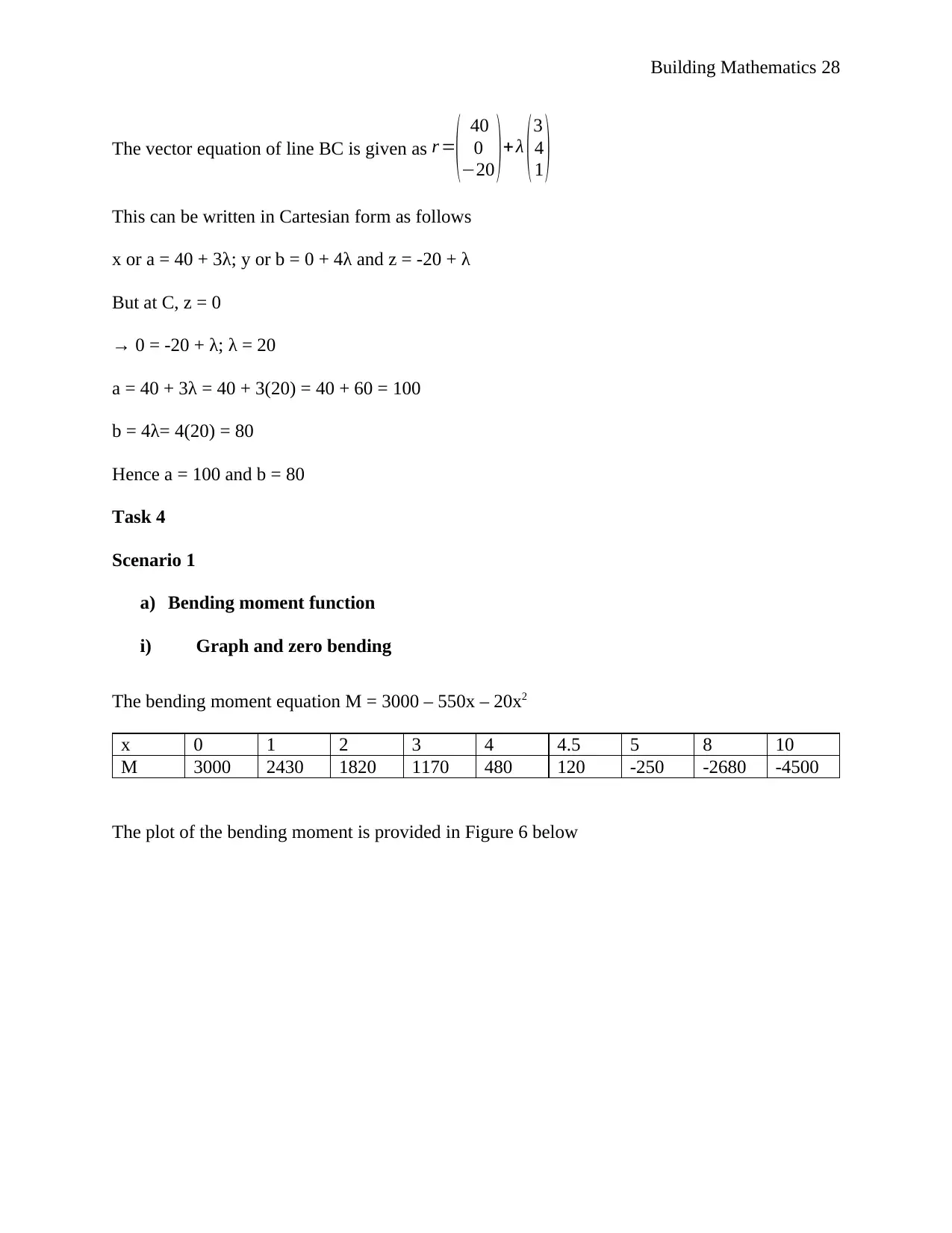
The vector equation of line BC is given as r =
( 40
0
−20 )+ λ (3
4
1 )
This can be written in Cartesian form as follows
x or a = 40 + 3λ; y or b = 0 + 4λ and z = -20 + λ
But at C, z = 0
→ 0 = -20 + λ; λ = 20
a = 40 + 3λ = 40 + 3(20) = 40 + 60 = 100
b = 4λ= 4(20) = 80
Hence a = 100 and b = 80
Task 4
Scenario 1
a) Bending moment function
i) Graph and zero bending
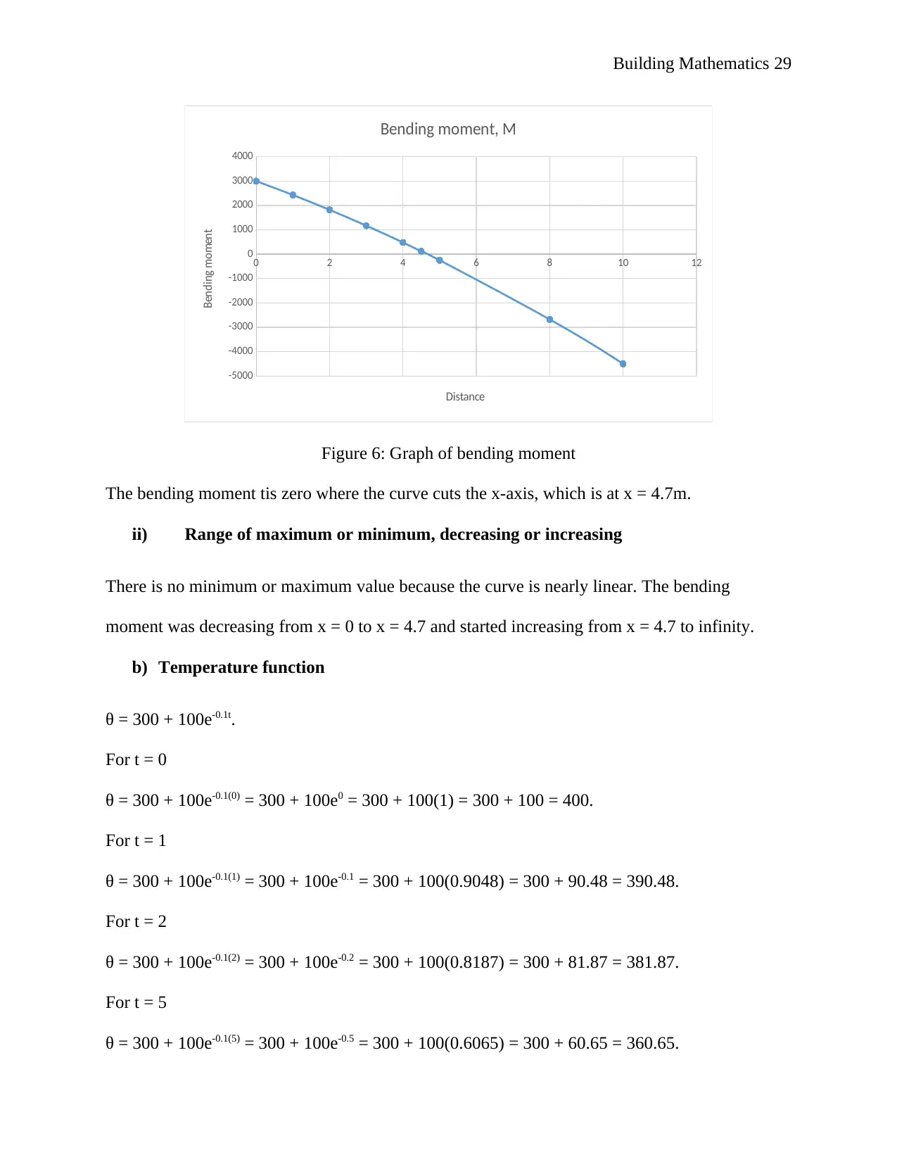
The bending moment equation M = 3000 – 550x – 20x2
x 0 1 2 3 4 4.5 5 8 10
M 3000 2430 1820 1170 480 120 -250 -2680 -4500
The plot of the bending moment is provided in Figure 6 below

Building Mathematics 29
0 2 4 6 8 10 12
-5000
-4000
-3000
-2000
-1000
0
1000
2000
3000
4000
Bending moment, M
Distance
Bending moment
Figure 6: Graph of bending moment
The bending moment tis zero where the curve cuts the x-axis, which is at x = 4.7m.
ii) Range of maximum or minimum, decreasing or increasing
There is no minimum or maximum value because the curve is nearly linear. The bending
moment was decreasing from x = 0 to x = 4.7 and started increasing from x = 4.7 to infinity.
b) Temperature function
θ = 300 + 100e-0.1t.
For t = 0
θ = 300 + 100e-0.1(0) = 300 + 100e0 = 300 + 100(1) = 300 + 100 = 400.
For t = 1
θ = 300 + 100e-0.1(1) = 300 + 100e-0.1 = 300 + 100(0.9048) = 300 + 90.48 = 390.48.
For t = 2
θ = 300 + 100e-0.1(2) = 300 + 100e-0.2 = 300 + 100(0.8187) = 300 + 81.87 = 381.87.
For t = 5
θ = 300 + 100e-0.1(5) = 300 + 100e-0.5 = 300 + 100(0.6065) = 300 + 60.65 = 360.65.

Building Mathematics 30
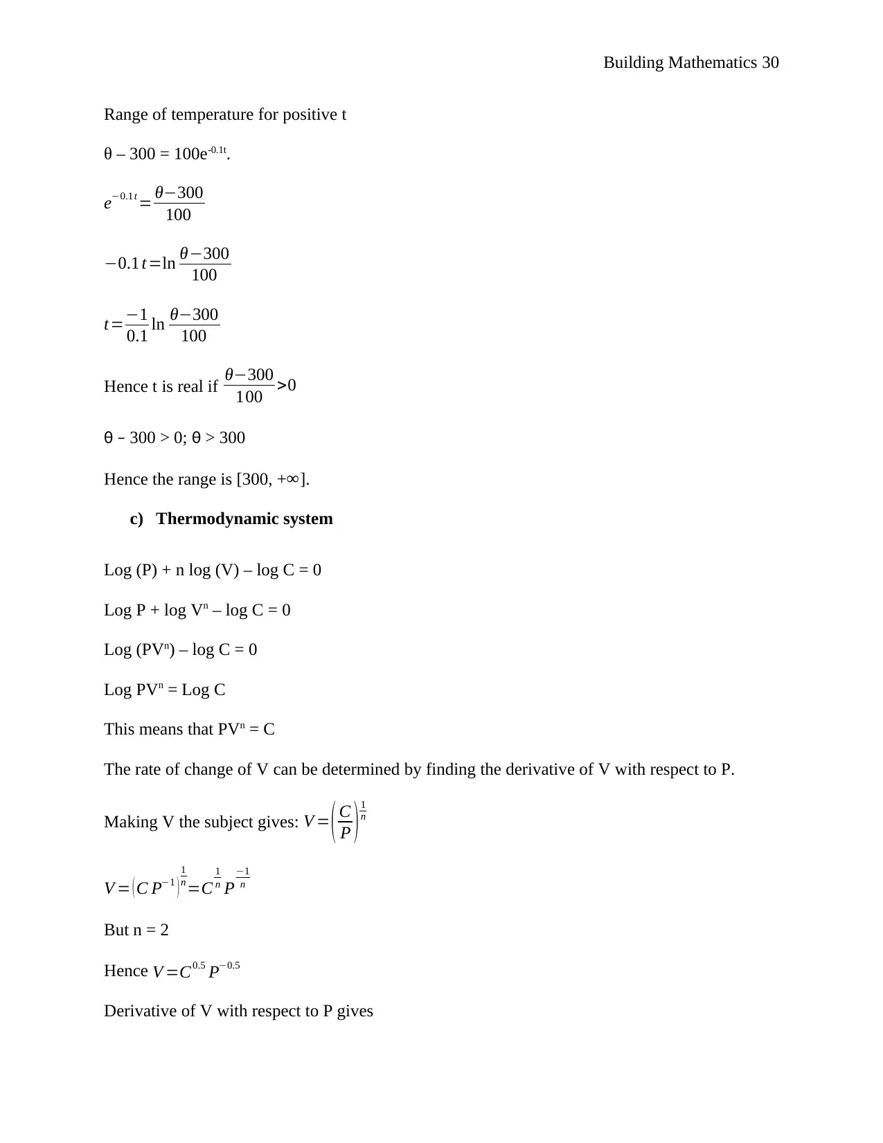
Range of temperature for positive t
θ – 300 = 100e-0.1t.
e−0.1t = θ−300
100
−0.1 t =ln θ−300
100
t=−1
0.1 ln θ−300
100
Hence t is real if θ−300
100 >0
θ – 300 > 0; θ > 300
Hence the range is [300, +∞].
c) Thermodynamic system
Log (P) + n log (V) – log C = 0
Log P + log Vn – log C = 0
Log (PVn) – log C = 0
Log PVn = Log C
This means that PVn = C
The rate of change of V can be determined by finding the derivative of V with respect to P.
Making V the subject gives: V = ( C
P ) 1
n
V = ( C P−1 )
1
n =C
1
n P
−1
n
But n = 2
Hence V =C0.5 P−0.5
Derivative of V with respect to P gives

Building Mathematics 31
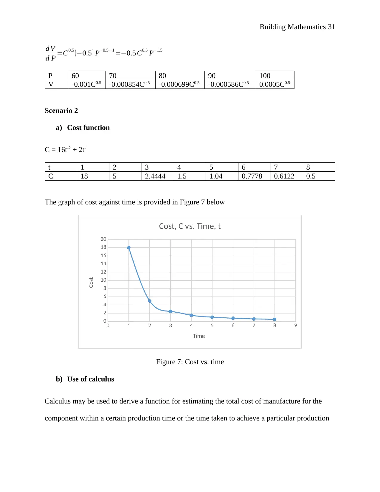
d V
d P =C0.5 ( −0.5 ) P−0.5 −1 =−0.5 C0.5 P−1.5
P 60 70 80 90 100
V -0.001C0.5 -0.000854C0.5 -0.000699C0.5 -0.000586C0.5 0.0005C0.5
Scenario 2
a) Cost function
C = 16t-2 + 2t-1
t 1 2 3 4 5 6 7 8
C 18 5 2.4444 1.5 1.04 0.7778 0.6122 0.5
The graph of cost against time is provided in Figure 7 below
0 1 2 3 4 5 6 7 8 9
0
2
4
6
8
10
12
14
16
18
20
Cost, C vs. Time, t
Time
Cost
Figure 7: Cost vs. time
b) Use of calculus
Calculus may be used to derive a function for estimating the total cost of manufacture for the
component within a certain production time or the time taken to achieve a particular production

Building Mathematics 32
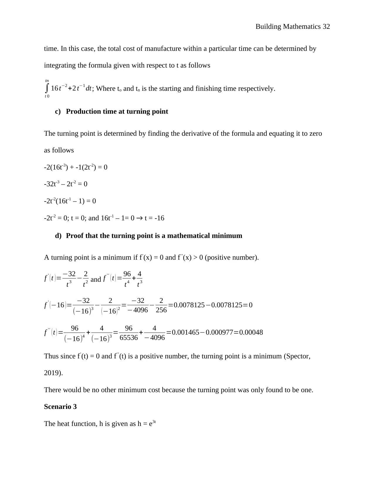
time. In this case, the total cost of manufacture within a particular time can be determined by
integrating the formula given with respect to t as follows
∫
t 0
tn
16 t−2 +2 t−1 dt; Where to and tn is the starting and finishing time respectively.
c) Production time at turning point
The turning point is determined by finding the derivative of the formula and equating it to zero
as follows
-2(16t-3) + -1(2t-2) = 0
-32t-3 – 2t-2 = 0
-2t-2(16t-1 – 1) = 0
-2t-2 = 0; t = 0; and 16t-1 – 1= 0 → t = -16
d) Proof that the turning point is a mathematical minimum
A turning point is a minimum if f’(x) = 0 and f’’(x) > 0 (positive number).
f ' ( t ) =−32
t3 − 2
t2 and f ' ' ( t ) = 96
t4 + 4
t 3
f ' ( −16 ) = −32
(−16)3 − 2
( −16 ) 2 = −32
−4096 − 2
256 =0.0078125−0.0078125=0
f '' ( t ) = 96
(−16)4 + 4
(−16)3 = 96
65536 + 4
−4096 =0.001465−0.000977=0.00048
Thus since f’(t) = 0 and f’’(t) is a positive number, the turning point is a minimum (Spector,
2019).
There would be no other minimum cost because the turning point was only found to be one.
Scenario 3
The heat function, h is given as h = e3t

Building Mathematics 33
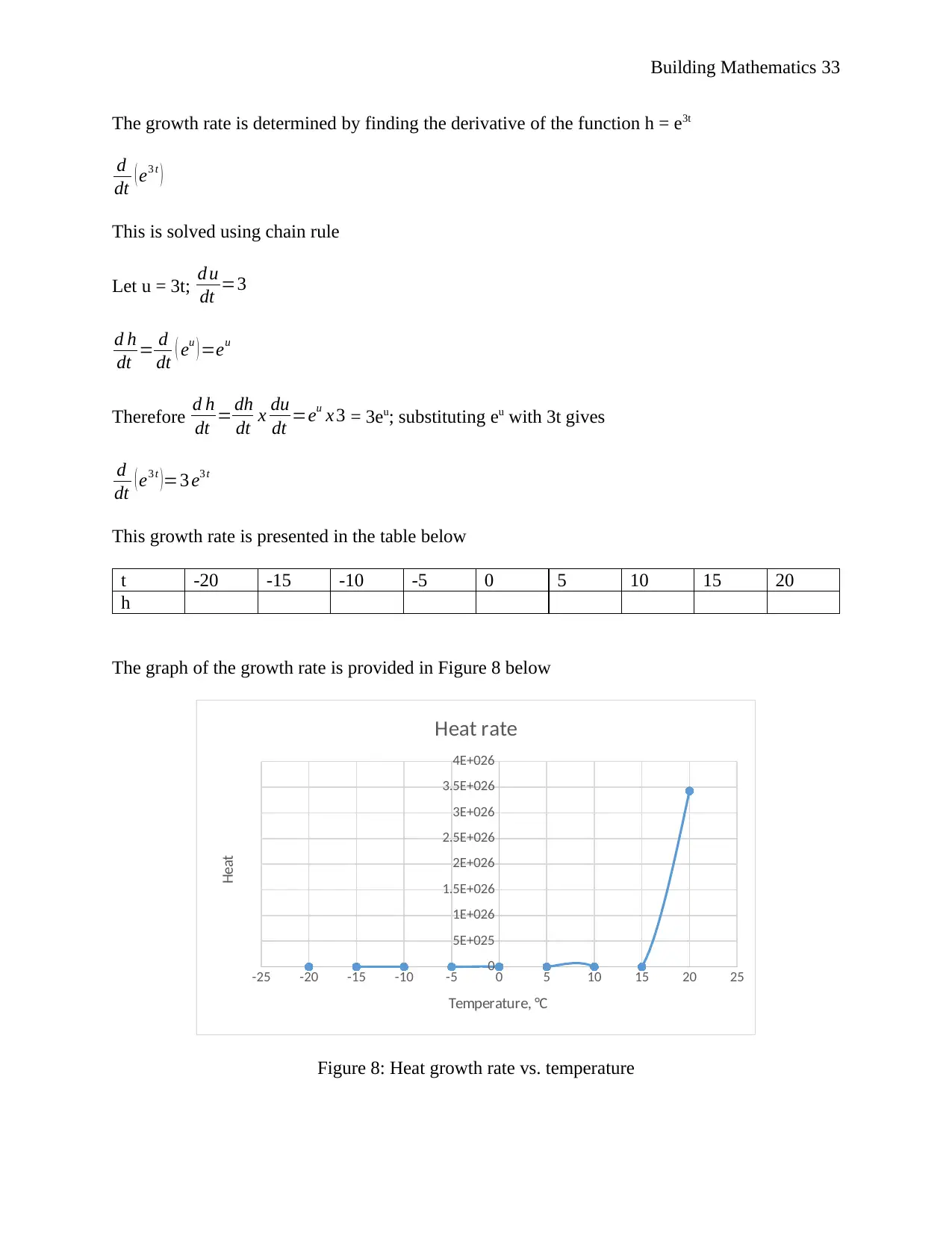
The growth rate is determined by finding the derivative of the function h = e3t
d
dt ( e3 t )
This is solved using chain rule
Let u = 3t; d u
dt =3
d h
dt = d
dt ( eu ) =eu
Therefore d h
dt = dh
dt x du
dt =eu x 3 = 3eu; substituting eu with 3t gives
d
dt ( e3 t )=3 e3 t
This growth rate is presented in the table below
t -20 -15 -10 -5 0 5 10 15 20
h
The graph of the growth rate is provided in Figure 8 below
-25 -20 -15 -10 -5 0 5 10 15 20 25
0
5E+025
1E+026
1.5E+026
2E+026
2.5E+026
3E+026
3.5E+026
4E+026
Heat rate
Temperature, °C
Heat
Figure 8: Heat growth rate vs. temperature

Building Mathematics 34
References
Hit Bullseye, 2019. Quick Review: Arithmetic, Geometric and Harmonic Progressions. [Online]
Available at: https://www.hitbullseye.com/Quant/Arithmetic-Geometric-Harmonic-
Progressions.php
[Accessed 4 May 2019].
Kean University, (n.d.). Hypothesis Testing of a Single Population Mean. [Online]
Available at: https://www.kean.edu/~fosborne/bstat/07amean.html
[Accessed 4 May 2019].
Lane, D., (n.d.). Introduction to Normal Distributions. [Online]
Available at: http://onlinestatbook.com/2/normal_distribution/intro.html
[Accessed 4 May 2019].
Lumen, (n.d.). Geometric Sequences and Series. [Online]
Available at: https://courses.lumenlearning.com/boundless-algebra/chapter/geometric-sequences-
and-series/
[Accessed 3 May 2019].
Spector, L., 2019. Maximum and Minimum Values. [Online]
Available at: https://www.themathpage.com/aCalc/max.htm
[Accessed 4 May 2019].