Impact of Taxes on Alcops Market
VerifiedAdded on 2020/02/24
|12
|1698
|97
AI Summary
This assignment delves into the consequences of imposing a tax on Alcops, a hypothetical alcoholic beverage. It begins by illustrating how the tax affects market equilibrium, leading to higher prices for consumers and lower revenue for producers. The analysis then focuses on the distribution of the tax burden between buyers and sellers, considering the elasticity of demand and supply. The assignment concludes with suggestions for government policies aimed at reducing Alcops consumption, emphasizing public awareness campaigns and educational initiatives.
Contribute Materials
Your contribution can guide someone’s learning journey. Share your
documents today.
Running head: MICROECONOMICS
Microeconomics
Name of the Student
Name of the University
Author note
Microeconomics
Name of the Student
Name of the University
Author note
Secure Best Marks with AI Grader
Need help grading? Try our AI Grader for instant feedback on your assignments.
1
MICROECONOMICS
Table of Contents
Question 1........................................................................................................................................2
Question 2........................................................................................................................................5
Part I.............................................................................................................................................5
Part II...........................................................................................................................................5
Question 3......................................................................................................................................10
References......................................................................................................................................12
2
MICROECONOMICS
Question 1
a)
0 5000 10000 15000 20000 25000 30000 35000
0
1000
2000
3000
4000
5000
6000
Production Possibility Curve
Cars
Bicycles
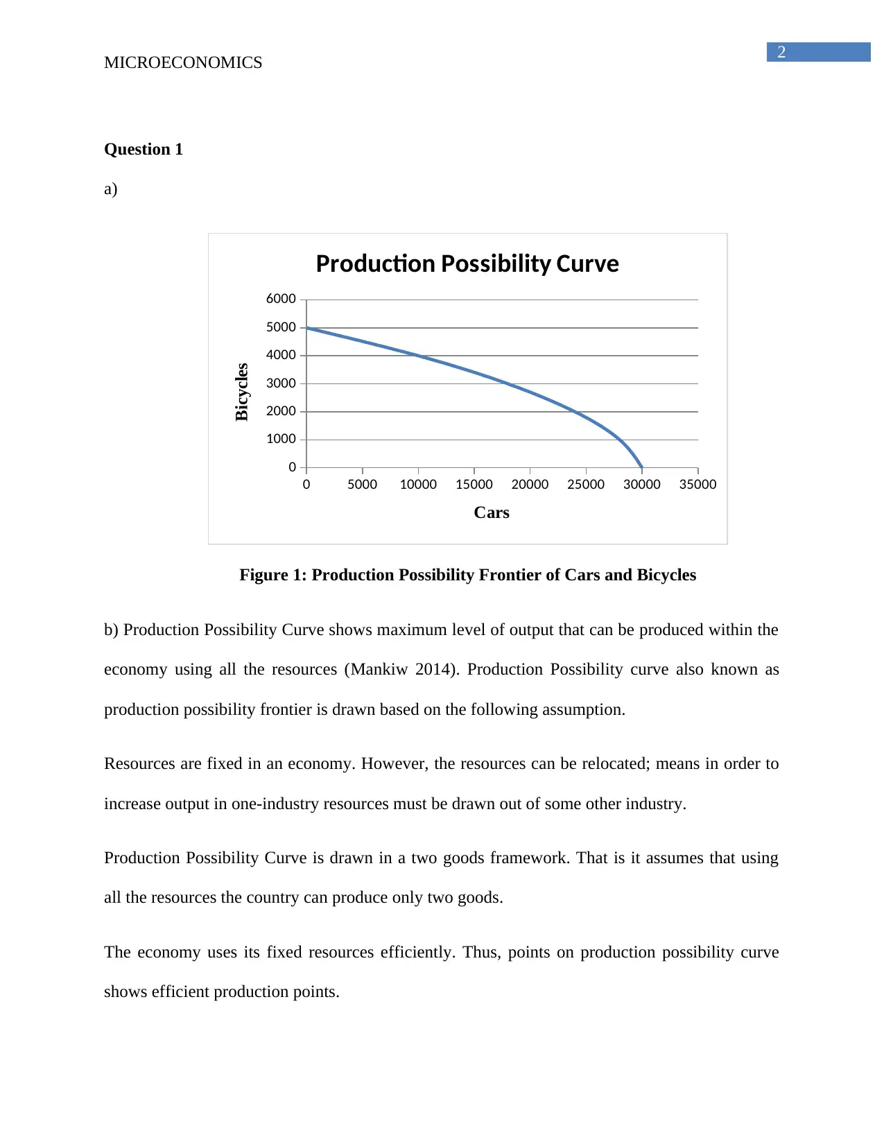
Figure 1: Production Possibility Frontier of Cars and Bicycles
b) Production Possibility Curve shows maximum level of output that can be produced within the
economy using all the resources (Mankiw 2014). Production Possibility curve also known as
production possibility frontier is drawn based on the following assumption.
Resources are fixed in an economy. However, the resources can be relocated; means in order to
increase output in one-industry resources must be drawn out of some other industry.
Production Possibility Curve is drawn in a two goods framework. That is it assumes that using
all the resources the country can produce only two goods.
The economy uses its fixed resources efficiently. Thus, points on production possibility curve
shows efficient production points.
MICROECONOMICS
Question 1
a)
0 5000 10000 15000 20000 25000 30000 35000
0
1000
2000
3000
4000
5000
6000
Production Possibility Curve
Cars
Bicycles
Figure 1: Production Possibility Frontier of Cars and Bicycles
b) Production Possibility Curve shows maximum level of output that can be produced within the
economy using all the resources (Mankiw 2014). Production Possibility curve also known as
production possibility frontier is drawn based on the following assumption.
Resources are fixed in an economy. However, the resources can be relocated; means in order to
increase output in one-industry resources must be drawn out of some other industry.
Production Possibility Curve is drawn in a two goods framework. That is it assumes that using
all the resources the country can produce only two goods.
The economy uses its fixed resources efficiently. Thus, points on production possibility curve
shows efficient production points.
3
MICROECONOMICS
Resources though moveable are however not equally efficient in producing all goods. This is the
reason when resources are shifted from one industry to another inefficiency increases (Nicholson
and Snyder 2014).
PPF is drawn assuming a constant level of technology.
PPC has the following characteristics.
i) PPC is downward sloping from left to right. Given limited resources, in order to increase
output of one good the country must sacrifice some other cost. This is called opportunity cost of
production.
ii) PPF is concave in shape to the origin. The opportunity cost involved in production operation
is increasing in nature. Not all resources are suitable for all industries (Findlay and Lundahl
2017). Hence, more the resources are drawn from specialized industry to the other industry the
opportunity cost increases.
c) In PPC, if demand for both goods increases simultaneously then this indicates point outside
the PPC, which is not feasible. The increased combination of cars and bicycles are obtained only
when there is a shift in PPF implying an expansion of output capacity. Exploration of new
source of resource causes an expansion of output of both goods. When there is improvement in
technology used in both the industry then production in both the industry increases.
Specialization of resources to specific industries increases efficiency in resource use and hence
increases output of both goods. Newland can adapt either of the strategy to meet the new
demand.
Secure Best Marks with AI Grader
Need help grading? Try our AI Grader for instant feedback on your assignments.
4
MICROECONOMICS
Question 2
Part I
Price (dollars per
chip)
Quantity demanded (millions of chips per
year) Revenue
200 50 10000
250 45 11250
300 40 12000
350 35 12250
400 30 12000
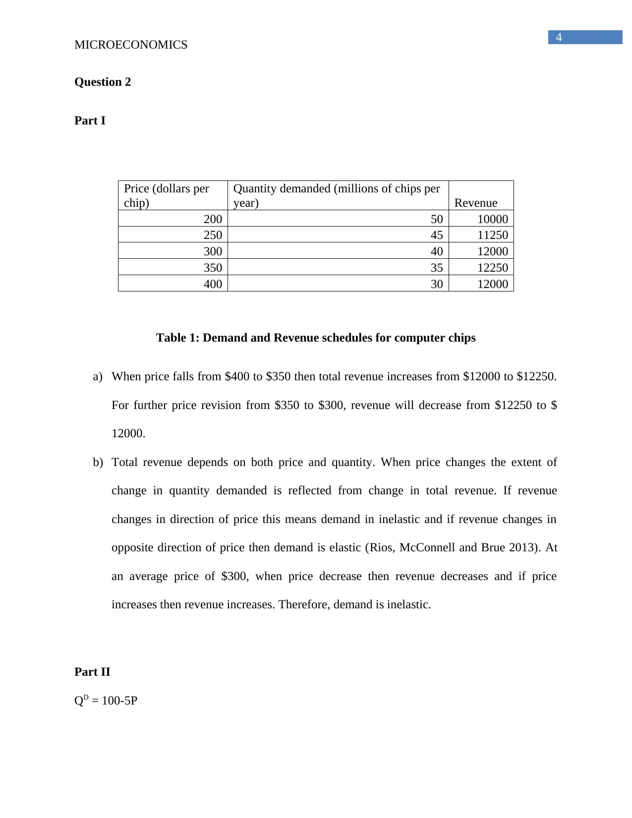
Table 1: Demand and Revenue schedules for computer chips
a) When price falls from $400 to $350 then total revenue increases from $12000 to $12250.
For further price revision from $350 to $300, revenue will decrease from $12250 to $
12000.
b) Total revenue depends on both price and quantity. When price changes the extent of
change in quantity demanded is reflected from change in total revenue. If revenue
changes in direction of price this means demand in inelastic and if revenue changes in
opposite direction of price then demand is elastic (Rios, McConnell and Brue 2013). At
an average price of $300, when price decrease then revenue decreases and if price
increases then revenue increases. Therefore, demand is inelastic.
Part II
QD = 100-5P
MICROECONOMICS
Question 2
Part I
Price (dollars per
chip)
Quantity demanded (millions of chips per
year) Revenue
200 50 10000
250 45 11250
300 40 12000
350 35 12250
400 30 12000
Table 1: Demand and Revenue schedules for computer chips
a) When price falls from $400 to $350 then total revenue increases from $12000 to $12250.
For further price revision from $350 to $300, revenue will decrease from $12250 to $
12000.
b) Total revenue depends on both price and quantity. When price changes the extent of
change in quantity demanded is reflected from change in total revenue. If revenue
changes in direction of price this means demand in inelastic and if revenue changes in
opposite direction of price then demand is elastic (Rios, McConnell and Brue 2013). At
an average price of $300, when price decrease then revenue decreases and if price
increases then revenue increases. Therefore, demand is inelastic.
Part II
QD = 100-5P
5
MICROECONOMICS
QS = 5P
c) At equilibrium, demand equals supply.
QD = QS
Or, 100-5P= 5P
Or, 5P+5P= 100
Or, 10P=100
Or, P= 10
Q = 5P = (5*10) = 50.
Equilibrium price is 10 and corresponding equilibrium quantity is 50.
d)Consumer surplus = Area of the triangle above the equilibrium price and below the maximum
price that consumers willing to pay (Wadman 2016).
The maximum price consumer willing to pay is derived from the demand curve as-
QD = 100-5P
When QD=0, then P = (100/5) = 20. This is the maximum price that the consumers willing to pay.
Therefore,CS=1
2∗( 20−10 )∗50= 1
2∗10∗50=250
Producer surplus= Area of the triangle above the minimum price that the suppliers and below the
equilibrium price (Heslop 2014).
The minimum price that the suppliers charge is obtained from the given supply equation,
6
MICROECONOMICS
QS = 5P, pitting QS = 0, minimum supply price P is obtained as P= 0/5=0
Therefore, PS=1
2∗( 10−0 )∗50= 1
2∗10∗50=250
Total Surplus=consumer surplus+ produc er surplus
¿ 250+250=500
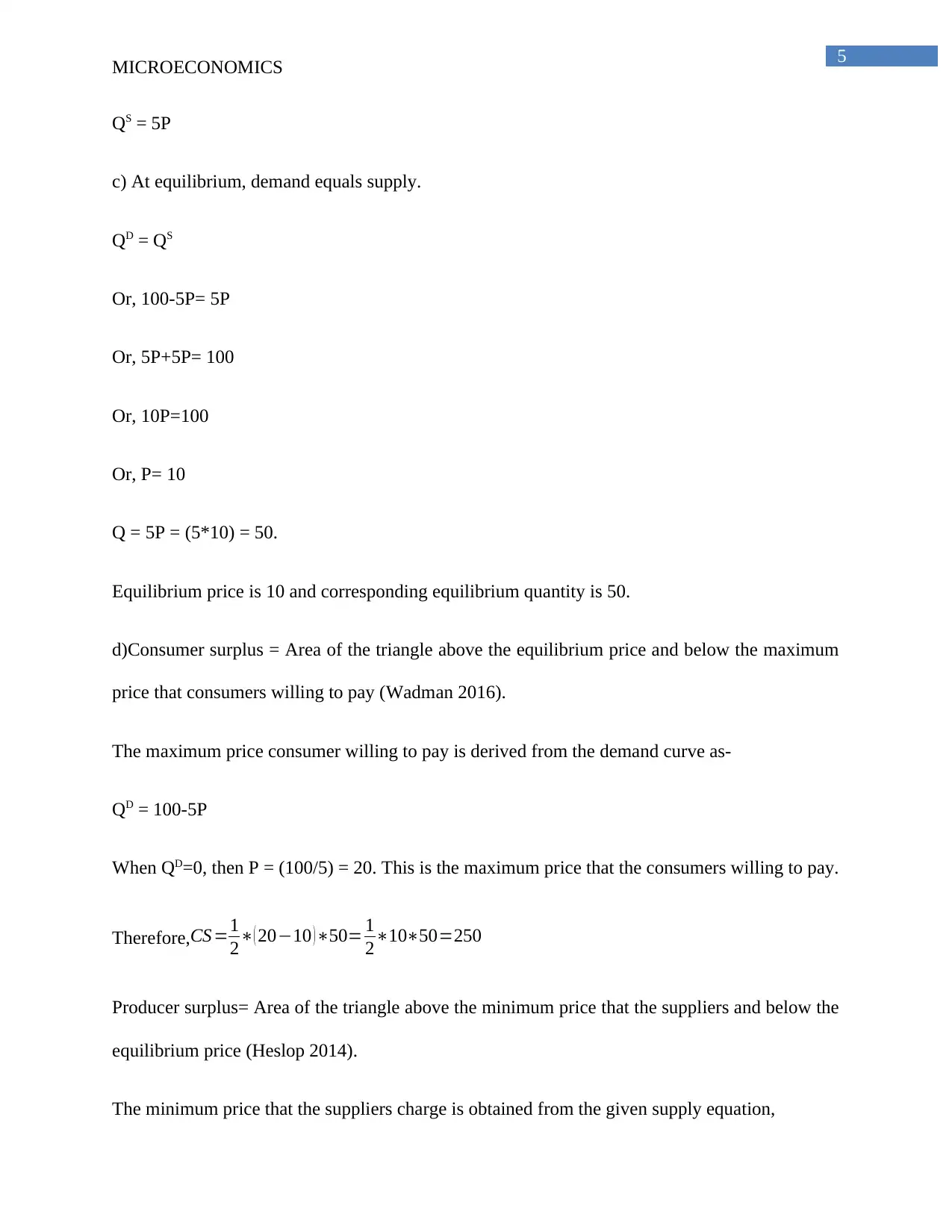
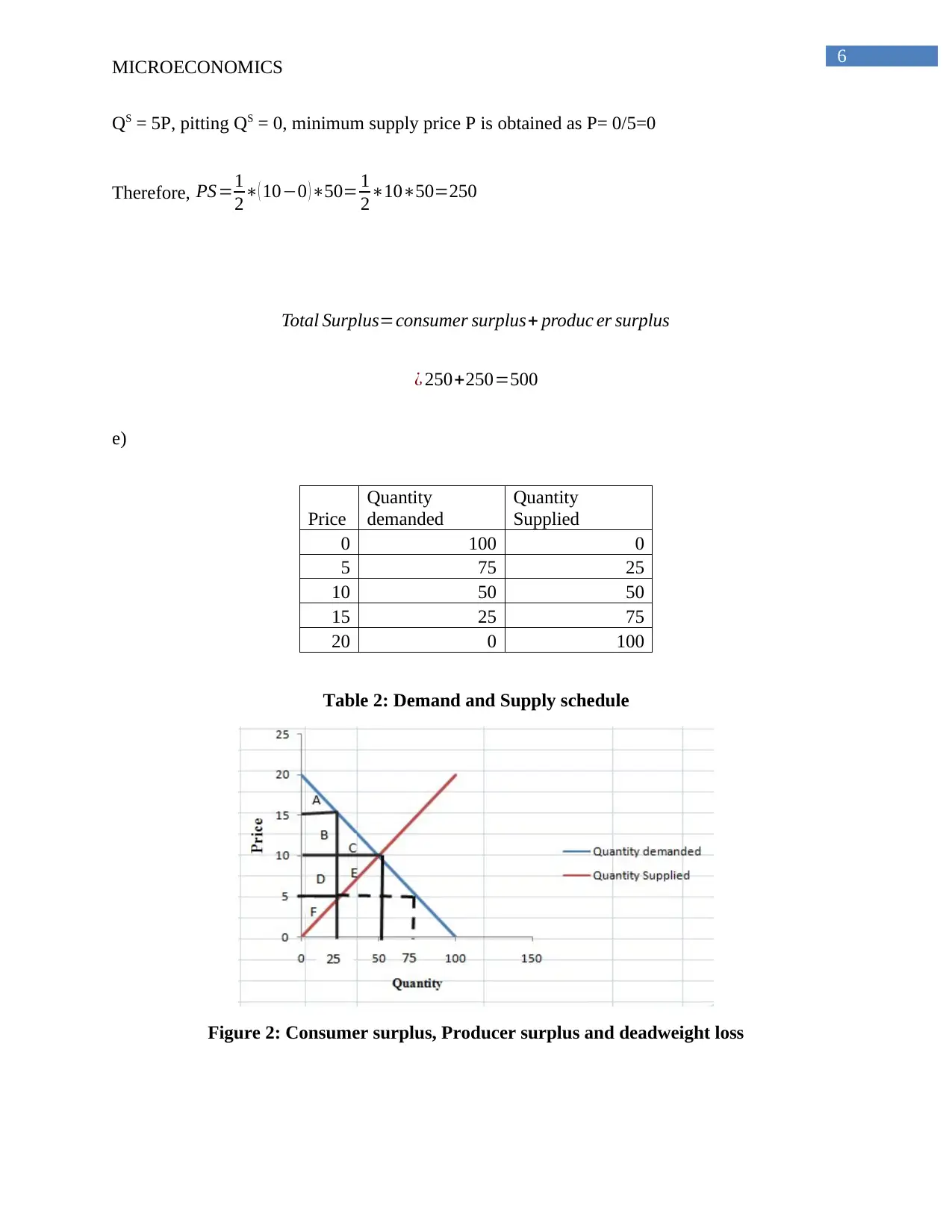
e)
Price
Quantity
demanded
Quantity
Supplied
0 100 0
5 75 25
10 50 50
15 25 75
20 0 100
Table 2: Demand and Supply schedule
Figure 2: Consumer surplus, Producer surplus and deadweight loss
MICROECONOMICS
QS = 5P, pitting QS = 0, minimum supply price P is obtained as P= 0/5=0
Therefore, PS=1
2∗( 10−0 )∗50= 1
2∗10∗50=250
Total Surplus=consumer surplus+ produc er surplus
¿ 250+250=500
e)
Price
Quantity
demanded
Quantity
Supplied
0 100 0
5 75 25
10 50 50
15 25 75
20 0 100
Table 2: Demand and Supply schedule
Figure 2: Consumer surplus, Producer surplus and deadweight loss
Paraphrase This Document
Need a fresh take? Get an instant paraphrase of this document with our AI Paraphraser
7
MICROECONOMICS
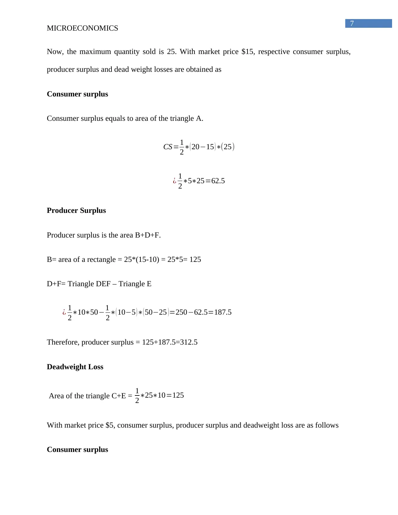
Now, the maximum quantity sold is 25. With market price $15, respective consumer surplus,
producer surplus and dead weight losses are obtained as
Consumer surplus
Consumer surplus equals to area of the triangle A.
CS=1
2∗( 20−15 )∗(25)
¿ 1
2∗5∗25=62.5
Producer Surplus
Producer surplus is the area B+D+F.
B= area of a rectangle = 25*(15-10) = 25*5= 125
D+F= Triangle DEF – Triangle E
¿ 1
2∗10∗50−1
2∗( 10−5 )∗( 50−25 )=250−62.5=187.5
Therefore, producer surplus = 125+187.5=312.5
Deadweight Loss
Area of the triangle C+E = 1
2∗25∗10=125
With market price $5, consumer surplus, producer surplus and deadweight loss are as follows
Consumer surplus
MICROECONOMICS
Now, the maximum quantity sold is 25. With market price $15, respective consumer surplus,
producer surplus and dead weight losses are obtained as
Consumer surplus
Consumer surplus equals to area of the triangle A.
CS=1
2∗( 20−15 )∗(25)
¿ 1
2∗5∗25=62.5
Producer Surplus
Producer surplus is the area B+D+F.
B= area of a rectangle = 25*(15-10) = 25*5= 125
D+F= Triangle DEF – Triangle E
¿ 1
2∗10∗50−1
2∗( 10−5 )∗( 50−25 )=250−62.5=187.5
Therefore, producer surplus = 125+187.5=312.5
Deadweight Loss
Area of the triangle C+E = 1
2∗25∗10=125
With market price $5, consumer surplus, producer surplus and deadweight loss are as follows
Consumer surplus
8
MICROECONOMICS
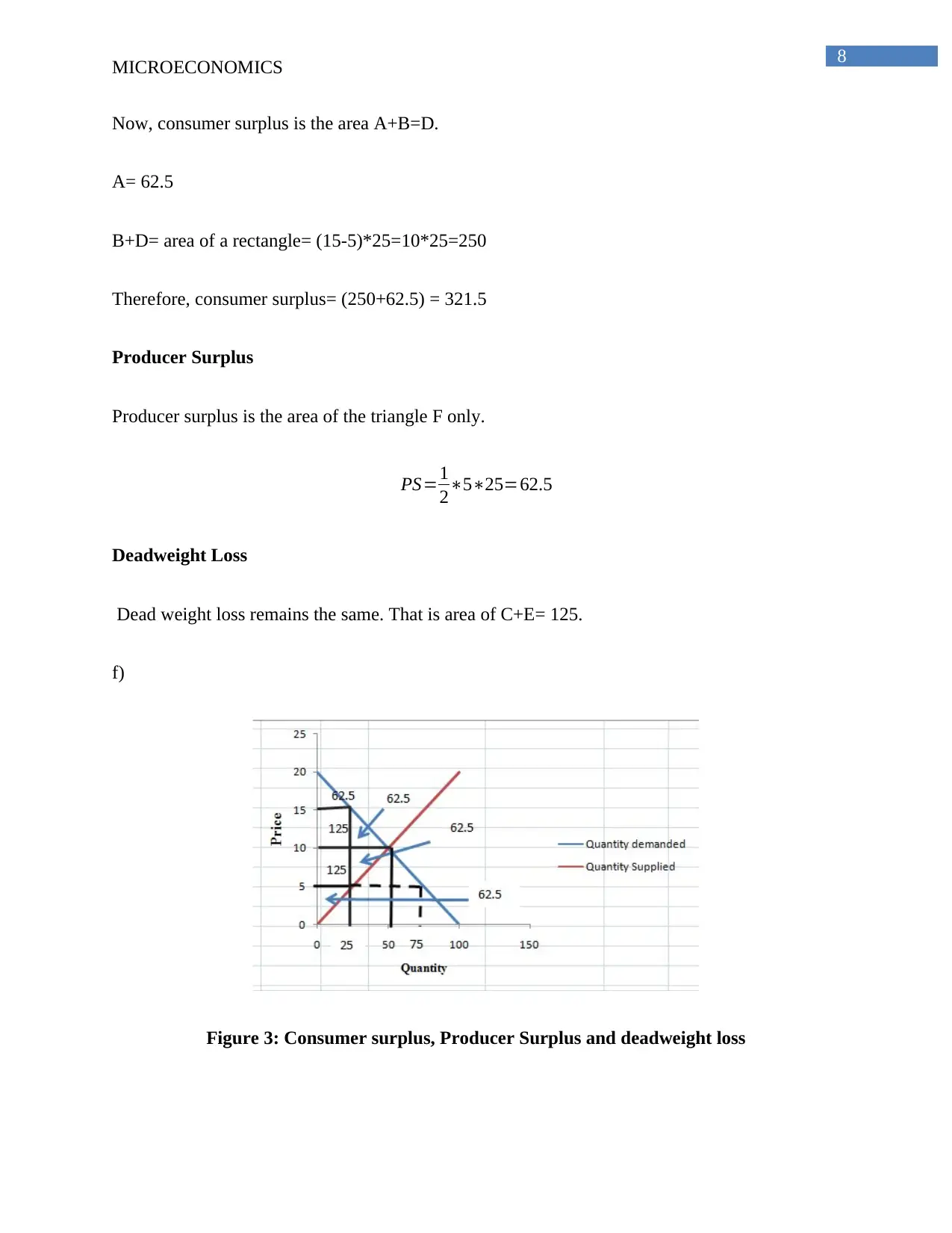
Now, consumer surplus is the area A+B=D.
A= 62.5
B+D= area of a rectangle= (15-5)*25=10*25=250
Therefore, consumer surplus= (250+62.5) = 321.5
Producer Surplus
Producer surplus is the area of the triangle F only.
PS=1
2∗5∗25=62.5
Deadweight Loss
Dead weight loss remains the same. That is area of C+E= 125.
f)
Figure 3: Consumer surplus, Producer Surplus and deadweight loss
MICROECONOMICS
Now, consumer surplus is the area A+B=D.
A= 62.5
B+D= area of a rectangle= (15-5)*25=10*25=250
Therefore, consumer surplus= (250+62.5) = 321.5
Producer Surplus
Producer surplus is the area of the triangle F only.
PS=1
2∗5∗25=62.5
Deadweight Loss
Dead weight loss remains the same. That is area of C+E= 125.
f)
Figure 3: Consumer surplus, Producer Surplus and deadweight loss
9
MICROECONOMICS
Question 3
a)
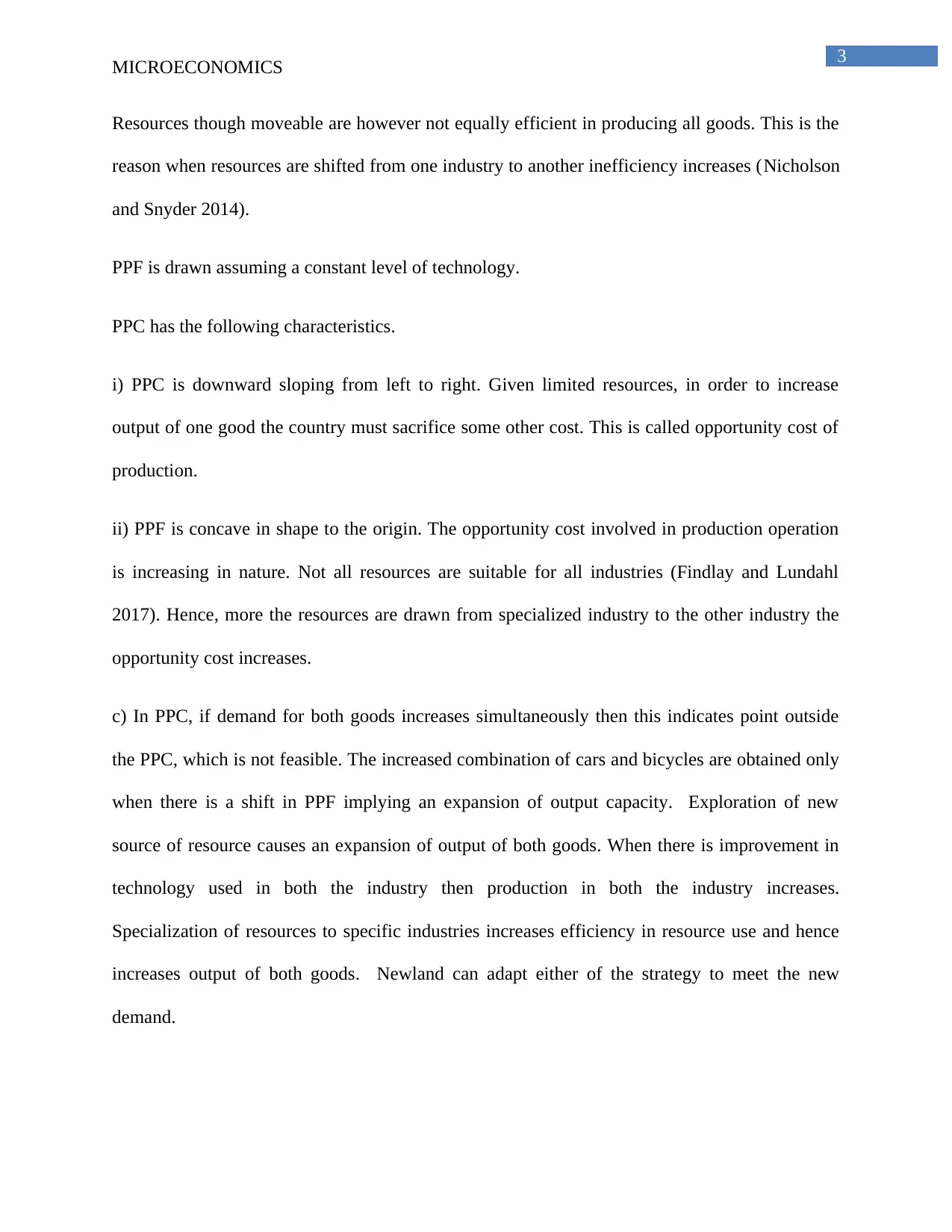
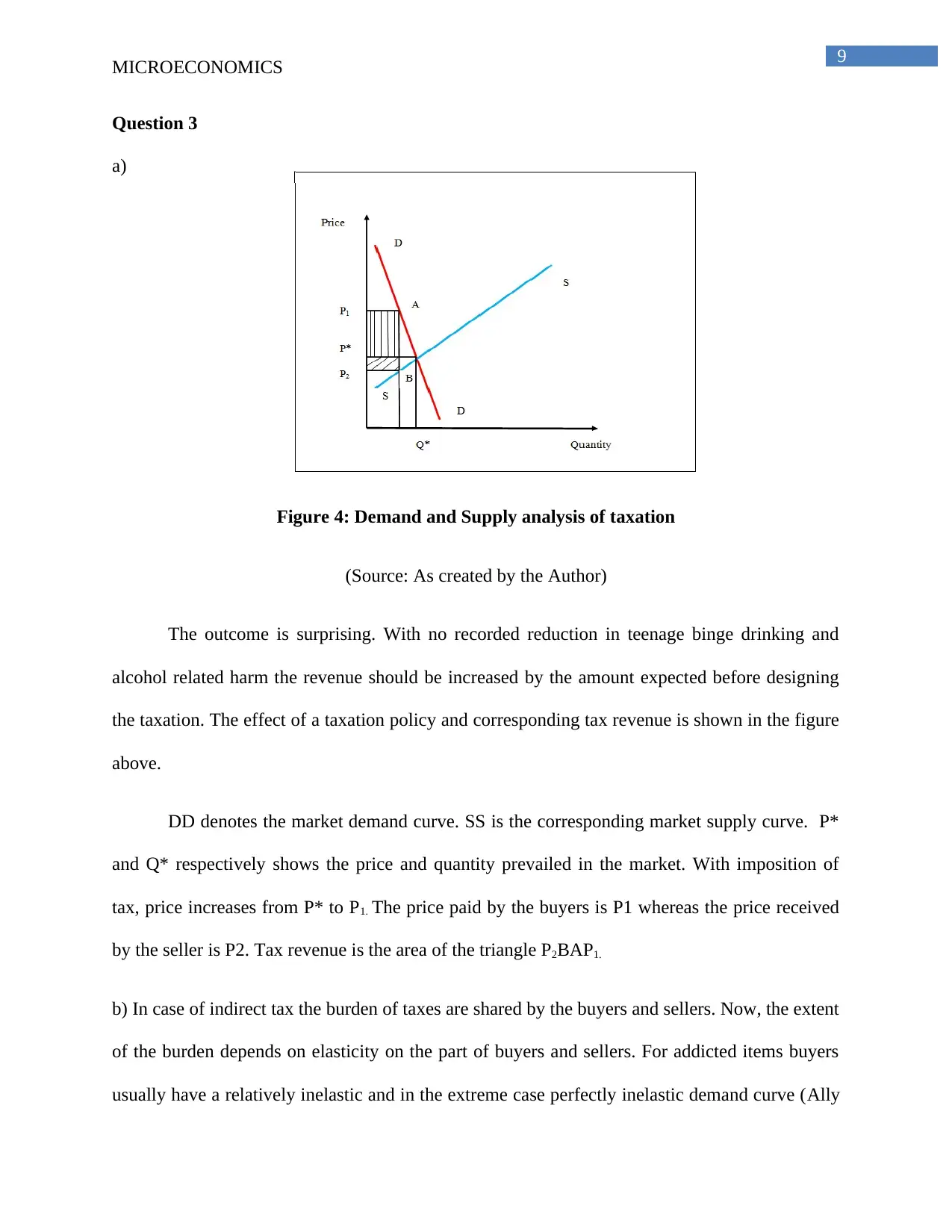
Figure 4: Demand and Supply analysis of taxation
(Source: As created by the Author)
The outcome is surprising. With no recorded reduction in teenage binge drinking and
alcohol related harm the revenue should be increased by the amount expected before designing
the taxation. The effect of a taxation policy and corresponding tax revenue is shown in the figure
above.
DD denotes the market demand curve. SS is the corresponding market supply curve. P*
and Q* respectively shows the price and quantity prevailed in the market. With imposition of
tax, price increases from P* to P1. The price paid by the buyers is P1 whereas the price received
by the seller is P2. Tax revenue is the area of the triangle P2BAP1.
b) In case of indirect tax the burden of taxes are shared by the buyers and sellers. Now, the extent
of the burden depends on elasticity on the part of buyers and sellers. For addicted items buyers
usually have a relatively inelastic and in the extreme case perfectly inelastic demand curve (Ally
MICROECONOMICS
Question 3
a)
Figure 4: Demand and Supply analysis of taxation
(Source: As created by the Author)
The outcome is surprising. With no recorded reduction in teenage binge drinking and
alcohol related harm the revenue should be increased by the amount expected before designing
the taxation. The effect of a taxation policy and corresponding tax revenue is shown in the figure
above.
DD denotes the market demand curve. SS is the corresponding market supply curve. P*
and Q* respectively shows the price and quantity prevailed in the market. With imposition of
tax, price increases from P* to P1. The price paid by the buyers is P1 whereas the price received
by the seller is P2. Tax revenue is the area of the triangle P2BAP1.
b) In case of indirect tax the burden of taxes are shared by the buyers and sellers. Now, the extent
of the burden depends on elasticity on the part of buyers and sellers. For addicted items buyers
usually have a relatively inelastic and in the extreme case perfectly inelastic demand curve (Ally
Secure Best Marks with AI Grader
Need help grading? Try our AI Grader for instant feedback on your assignments.
10
MICROECONOMICS
et al. 2014). As there are no recorded reduction in drinking it implies the demand remains more
or less same. In case of inelastic depend sellers are able to pass maximum burden to the buyers.
In the above figure the smaller rectangle shows burden to the seller and the larger rectangle
shows burden to buyers. It is clearly explained from the diagram that buyers of Alcops bore the
greater burden.
The tax outcome is not efficient. The tax is intended to affect both the buyers and sellers
and hence reduce the consumption of Alcops in a comprehensive way (Colchero et al. 2015). As
all the burdens are bore by buyers there are no initiatives from sellers to reduce supply.
c) The government should arrange awareness program for increasing awareness about the
harmful impact Alcops and other alcohol related harm. Doctors, socialist, politicians all should
participate in the campaign. Most awareness is needed for the teenagers. The youth should be the
primary target of such campaign. Guidance can also be given to the parents to keep their children
safe from such harmful practices. Without active participation from all level it not possible to
completely eliminate such bad habits and other related harms for the individual and the society
as a whole.
11
MICROECONOMICS
References
Ally, A.K., Meng, Y., Chakraborty, R., Dobson, P.W., Seaton, J.S., Holmes, J., Angus, C., Guo,
Y., Hill‐McManus, D., Brennan, A. and Meier, P.S., 2014. Alcohol tax pass‐through across the
product and price range: do retailers treat cheap alcohol differently?. Addiction, 109(12),
pp.1994-2002.
Colchero, M.A., Salgado, J.C., Unar-Munguia, M., Hernandez-Avila, M. and Rivera-Dommarco,
J.A., 2015. Price elasticity of the demand for sugar sweetened beverages and soft drinks in
Mexico. Economics & Human Biology, 19, pp.129-137.
Findlay, R. and Lundahl, M., 2017. Towards a model of territorial expansion and the limits of
empire. In The Economics of the Frontier (pp. 105-124). Palgrave Macmillan UK.
Heslop, H., 2014. Theories of Surplus and Transfer (Routledge Revivals): Parasites and Producers
in Economic Thought. Routledge.
Mankiw, N.G., 2014. Principles of macroeconomics. Cengage Learning.
Nicholson, W. and Snyder, C.M., 2014. Intermediate microeconomics and its application.
Cengage Learning.
Rios, M.C., McConnell, C.R. and Brue, S.L., 2013. Economics: Principles, problems, and
policies. McGraw-Hill.
Wadman, W.M., 2016. Variable Quality in Consumer Theory: Towards a Dynamic
Microeconomic Theory of the Consumer. Routledge.
1 out of 12
Related Documents


Your All-in-One AI-Powered Toolkit for Academic Success.
+13062052269
info@desklib.com
Available 24*7 on WhatsApp / Email
![[object Object]](/_next/static/media/star-bottom.7253800d.svg)
Unlock your academic potential
© 2024 | Zucol Services PVT LTD | All rights reserved.