BUS105 Computing Assignment: Semester 3, 2017 - Variable Comparison

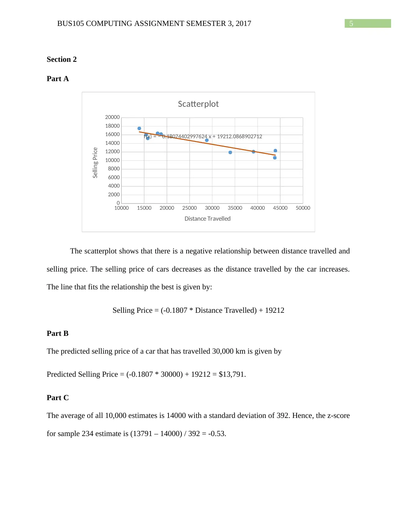
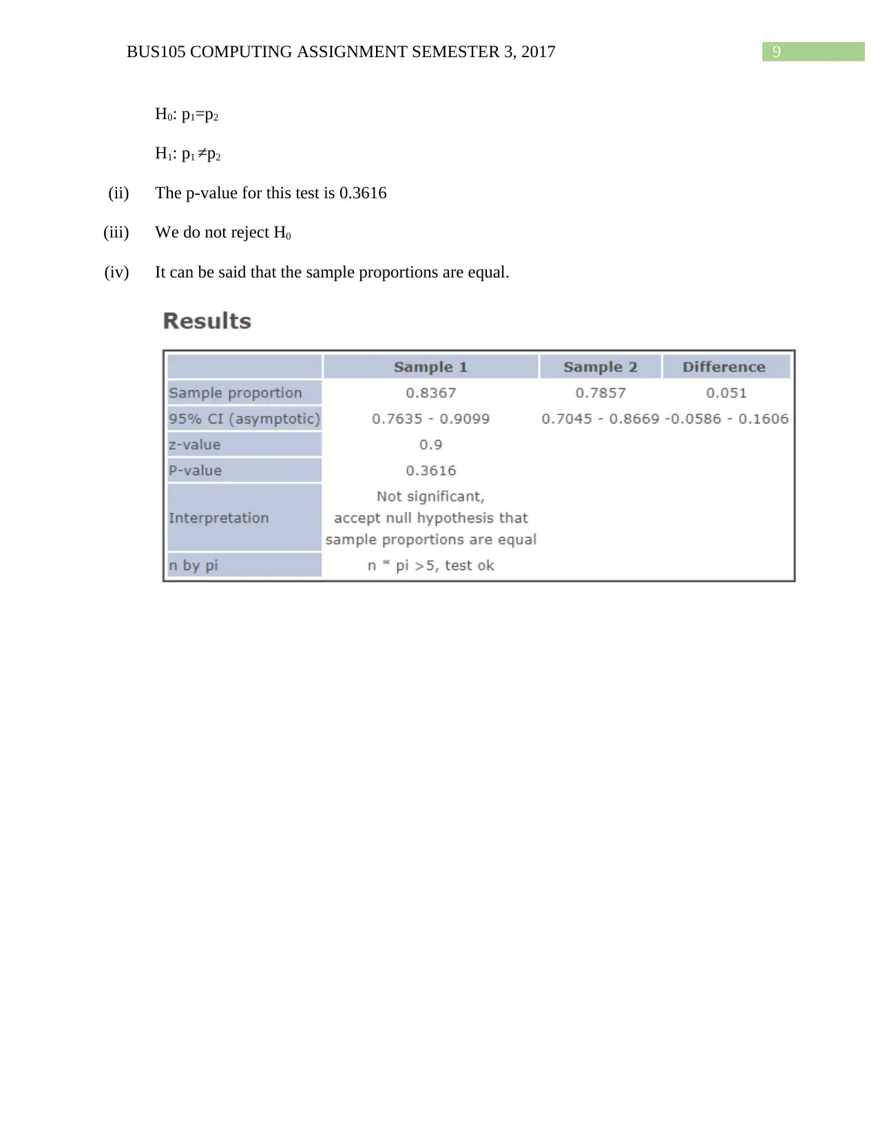
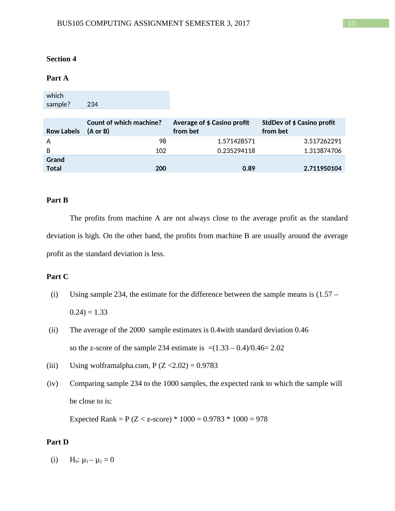
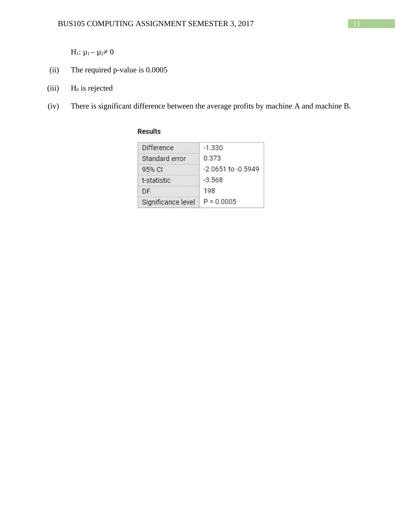
This BUS105 computing assignment from Semester 3, 2017, focuses on comparing different types of variables using data analysis techniques. The assignment explores the comparison of categorical and numerical variables, including the use of scatterplots to assess relationships between variables. The solution includes detailed analysis of sample data, calculating z-scores, and constructing confidence intervals. It also covers hypothesis testing to determine the significance of differences between sample means and proportions. The assignment uses various statistical methods to compare data, analyze the results, and draw conclusions, providing insights into practical data analysis applications. The analysis includes the use of tools like WolframAlpha to calculate probabilities and determine expected ranks. The assignment is a comprehensive examination of data analysis principles and their application.

Running Head: BUS105 COMPUTING ASSIGNMENT SEMESTER 3, 2017
BUS105 Computing Assignment Semester 3, 2017
Name of the Student
Student Number
Allocated Sample: 234

1BUS105 COMPUTING ASSIGNMENT SEMESTER 3, 2017
Executive Summary
Understanding the techniques that can be applied to compare different types of variables is the
main aim of this study. In the following sections, discussions will be made and applied for
comparisons of different types of variables.

2BUS105 COMPUTING ASSIGNMENT SEMESTER 3, 2017
Table of Contents
Section 1..........................................................................................................................................4
Section 2..........................................................................................................................................5
Part A...........................................................................................................................................5
Part B...........................................................................................................................................5
Part C...........................................................................................................................................5
Part D...........................................................................................................................................6
Part E...........................................................................................................................................6
Section 3..........................................................................................................................................7
Part A...........................................................................................................................................7
Part B...........................................................................................................................................7
Part C...........................................................................................................................................8
Part D...........................................................................................................................................8
Part E...........................................................................................................................................8
Section 4........................................................................................................................................10
Part A.........................................................................................................................................10
Part B.........................................................................................................................................10
Part C.........................................................................................................................................10
Part D.........................................................................................................................................10
Section 5........................................................................................................................................12

3BUS105 COMPUTING ASSIGNMENT SEMESTER 3, 2017
Section 6........................................................................................................................................13
Part A.........................................................................................................................................13
Part B.........................................................................................................................................13
Part C.........................................................................................................................................13
Part D.........................................................................................................................................13

4BUS105 COMPUTING ASSIGNMENT SEMESTER 3, 2017
Section 1
A dataset is a collection of information on a particular field. For example, information on
the names of the employees, the division in which they work and their salaries of a company will
be known as a dataset.
A dataset contains different variables which are usually compared among them. These
variables can be of two different types which are categorical and numerical. Categorical
variavles are the variables which represent some qualities and numeric variables are numbers
which vary according to situation. In the example stated above, division of working of the
employees are categorical and their salaries are numerical variables.
A categorical and a numerical variable can be compared by evaluating the average of the
numerical variables for each of the groups and comparing them. If two variables are numerical,
then their relationship would be assessed with the help of a scatter diagram. Two categorical
variables can be compared by evaluating their proportions.
Analysis and comparisons are done using computers as it reduces the efforts in making
the calculations and diagrams as well as reduces the time required to evaluate them.

5BUS105 COMPUTING ASSIGNMENT SEMESTER 3, 2017
Section 2
Part A
10000 15000 20000 25000 30000 35000 40000 45000 50000
0
2000
4000
6000
8000
10000
12000
14000
16000
18000
20000
f(x) = − 0.18074402997624 x + 19212.0868902712
Scatterplot
Distance Travelled
Selling Price
The scatterplot shows that there is a negative relationship between distance travelled and
selling price. The selling price of cars decreases as the distance travelled by the car increases.
The line that fits the relationship the best is given by:
Selling Price = (-0.1807 * Distance Travelled) + 19212
Part B
The predicted selling price of a car that has travelled 30,000 km is given by
Predicted Selling Price = (-0.1807 * 30000) + 19212 = $13,791.
Part C
The average of all 10,000 estimates is 14000 with a standard deviation of 392. Hence, the z-score
for sample 234 estimate is (13791 – 14000) / 392 = -0.53.

6BUS105 COMPUTING ASSIGNMENT SEMESTER 3, 2017
Part D
Using wolphramalphs.com, P (Z < -0.53) = 0.2981.
Part E
Comparing sample 234 with 10,000 samples, the sample rank will be close to:
Expected Rank = P (Z < z-score) * 10000 = 0.2981 * 10000 = 2981.

7BUS105 COMPUTING ASSIGNMENT SEMESTER 3, 2017
Section 3
Part A
which sample ? 234
Count of Do they like it ? (y=yes, n=no) Column Labels
Row Labels n y
Grand
Total
A 16 82 98
B 21 77 98
Grand Total 37
15
9 196
which sample ? 234
Count of Do they like it ? (y=yes, n=no) Column Labels
Row Labels n y
Grand
Total
A 16.33%
83.67
% 100.00%
B 21.43%
78.57
% 100.00%
Grand Total 18.88%
81.12
% 100.00%

8BUS105 COMPUTING ASSIGNMENT SEMESTER 3, 2017
Part B
Part C
Parts A and B show that version A is preferred over version B by most people.
Part D
(i) Using sample 234, the estimated difference in proportions is 0.8367 – 0.7857 = 0.051
(ii) The average of 1000 sample estimates is 0.1 with standard deviation 0.0505. Therefore,
the z-score for that estimate in sample 234 is (0.051– 0.1) / 0.0505 = -0.97
(iii) Using wolframalpha.com, P (Z < -0.97) = 0.1660
(iv) Comparing sample 234 to the 1000 samples, the expected rank to which the sample will
be close to is:
Expected Rank = P (Z < z-score) * 1000 = 0.1660 * 1000 = 166
Part E
(i) p1 is the proportion of people saying yes for version A and p2 is the proportion of people
saying yes for version B. Thus,

9BUS105 COMPUTING ASSIGNMENT SEMESTER 3, 2017
H0: p1=p2
H1: p1 ≠p2
(ii) The p-value for this test is 0.3616
(iii) We do not reject H0
(iv) It can be said that the sample proportions are equal.

10BUS105 COMPUTING ASSIGNMENT SEMESTER 3, 2017
Section 4
Part A
which
sample? 234
Row Labels
Count of which machine?
(A or B)
Average of $ Casino profit
from bet
StdDev of $ Casino profit
from bet
A 98 1.571428571 3.517262291
B 102 0.235294118 1.313874706
Grand
Total 200 0.89 2.711950104
Part B
The profits from machine A are not always close to the average profit as the standard
deviation is high. On the other hand, the profits from machine B are usually around the average
profit as the standard deviation is less.
Part C
(i) Using sample 234, the estimate for the difference between the sample means is (1.57 –
0.24) = 1.33
(ii) The average of the 2000 sample estimates is 0.4with standard deviation 0.46
so the z-score of the sample 234 estimate is =(1.33 – 0.4)/0.46= 2.02
(iii) Using wolframalpha.com, P (Z <2.02) = 0.9783
(iv) Comparing sample 234 to the 1000 samples, the expected rank to which the sample will
be close to is:
Expected Rank = P (Z < z-score) * 1000 = 0.9783 * 1000 = 978
Part D
(i) H0: μ1 – μ2 = 0

11BUS105 COMPUTING ASSIGNMENT SEMESTER 3, 2017
H1: μ1 – μ2≠ 0
(ii) The required p-value is 0.0005
(iii) H0 is rejected
(iv) There is significant difference between the average profits by machine A and machine B.