Comparative Analysis of Rental Properties in Four Suburbs

The assignment content provides an analysis of rental properties in four suburbs: Auburn, Parramatta, Randwick, and Sydney. The data reveals that flats are the most common dwelling type, with houses being less prevalent, particularly in Sydney. The weekly rent for two-bedroom dwellings varies across suburbs, with Sydney having the highest average weekly rent ($838.04) and Auburn having the lowest ($404.67). A strong linear correlation is found between bond amount and weekly rent, suggesting that the bond amount is typically equivalent to one month's rent. The analysis concludes that clients should consider these factors when searching for rental properties.

BUS708 STATISTICS
AND DATA ANALYSIS
STATISTICAL MODELLING ASSIGNMENT
STUDENT ID
[Pick the date]

Introduction
(a) The given company extends the service to those individuals who are coming to Australia
from various places of the world in order to fulfill various obligations. The company
provides accommodations either on permanent basis or on temporary basis. In this
regards, it is essential to determine the weekly rents pattern of the main four suburbs of
Australia i.e. Auburn, Parramatta, Randwick and Sydney based on the 500 sample data
collected from these suburbs. Further, the weekly rent amount pattern especially for the
international students would also be analyzed in the present report.
(b) Data set 1: The type of data collected for analyzing the weekly rent pattern for the
international students is primary data. This is because the data has been collected through
personal interview by asking the international student about their weekly rent. However,
there is possibility that the collected data set is biased because the sample data might not
be the true representative of population. This is because the data has not been collected
by considering the location, gender, financial status of the international student. Also, the
data has not been collected from a larger population and also the sample size is 20
students which are based on the convenience of the researcher. Further, weekly rent is a
quantitative data set and the scale of measurement for the data is ratio. This shows that
data has a well-defined zero and is numeric in nature.
(c) Data set 2: For the analysis, 500 samples have been collected from “Rental Bond Board
Property Data on Weekly Rent” for the four main suburbs from the “Department of
Finance.” This collected data would be termed as secondary data set because the data has
been collected from another data source. The collected data comprises weekly rent, bond
amount and number of bedrooms which is quantitative data set. Further, the suburb and
the dwelling type are the qualitative data. Ratio scale of measurement has been taken into
account for quantitative data and nominal scale of measurement has been used for
quantitative data set.
Analysis of weekly rent paid by International Student
(a) The descriptive statistics for the weekly rent paid by the international students is shown
below:
1

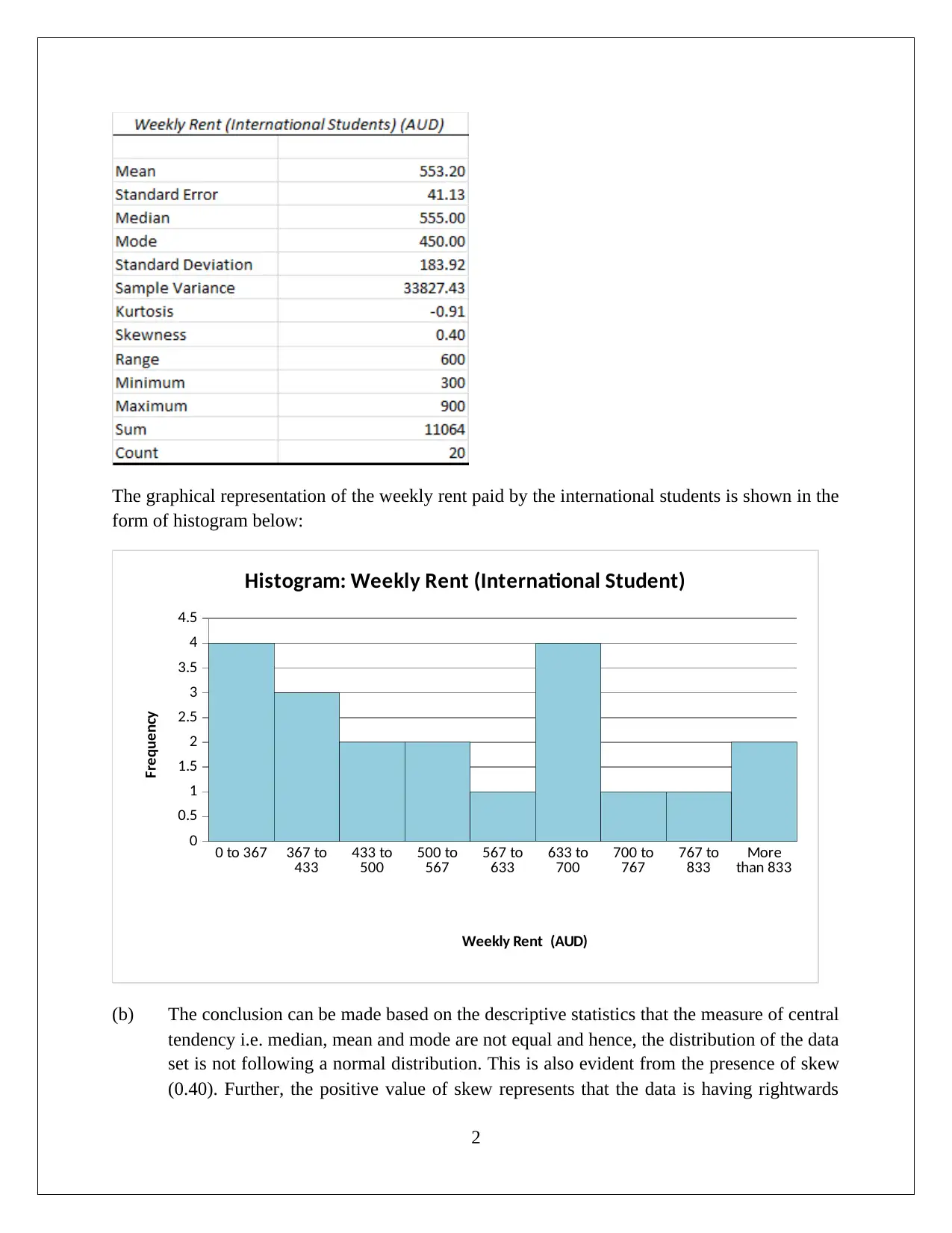
The graphical representation of the weekly rent paid by the international students is shown in the
form of histogram below:
0 to 367 367 to
433 433 to
500 500 to
567 567 to
633 633 to
700 700 to
767 767 to
833 More
than 833
0
0.5
1
1.5
2
2.5
3
3.5
4
4.5
Histogram: Weekly Rent (International Student)
Weekly Rent (AUD)
Frequency
(b) The conclusion can be made based on the descriptive statistics that the measure of central
tendency i.e. median, mean and mode are not equal and hence, the distribution of the data
set is not following a normal distribution. This is also evident from the presence of skew
(0.40). Further, the positive value of skew represents that the data is having rightwards
2

tail and also the existence of the outliers in the higher portion of the data. This is also
witnessed from the highlighted histogram (long tail in the rightward side). With regards
to the measures of dispersion, it can be said that standard deviation is on the lower side
when interpreted along the mean weekly rent.
“Rental Bond Board Property Data Set: Dwelling Type”
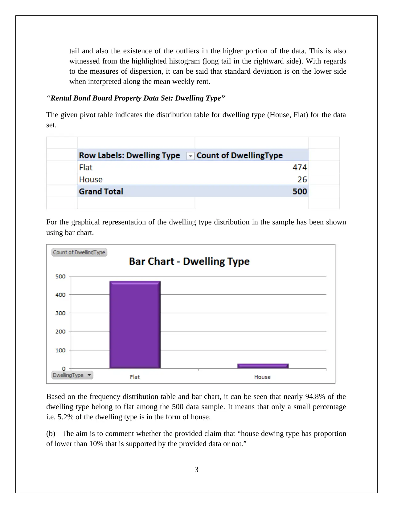
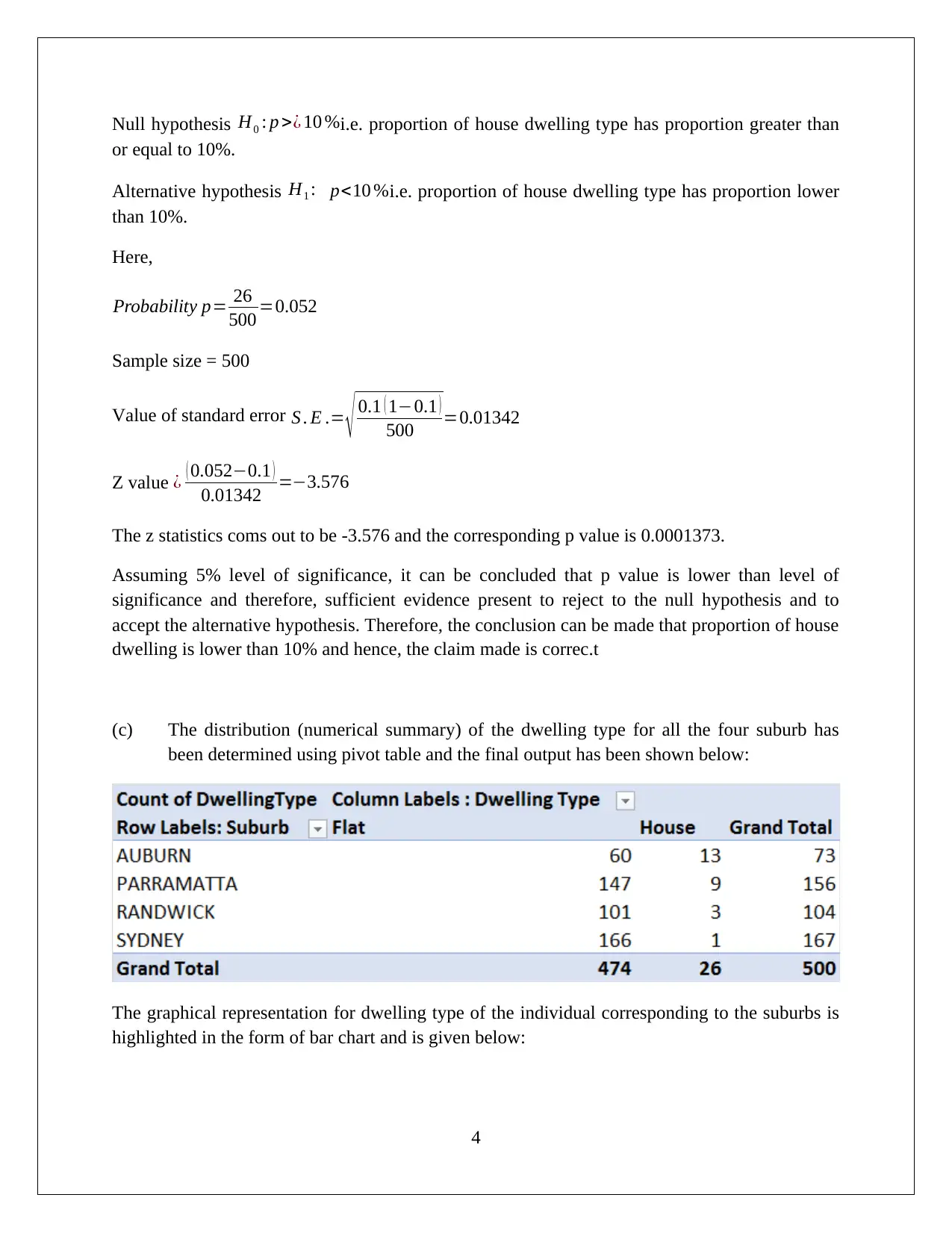
The given pivot table indicates the distribution table for dwelling type (House, Flat) for the data
set.
For the graphical representation of the dwelling type distribution in the sample has been shown
using bar chart.
Based on the frequency distribution table and bar chart, it can be seen that nearly 94.8% of the
dwelling type belong to flat among the 500 data sample. It means that only a small percentage
i.e. 5.2% of the dwelling type is in the form of house.
(b) The aim is to comment whether the provided claim that “house dewing type has proportion
of lower than 10% that is supported by the provided data or not.”
3

Null hypothesis H0 : p >¿ 10 %i.e. proportion of house dwelling type has proportion greater than
or equal to 10%.
Alternative hypothesis H1 : p<10 %i.e. proportion of house dwelling type has proportion lower
than 10%.
Here,
Probability p= 26
500 =0.052
Sample size = 500
Value of standard error S . E .= √ 0.1 ( 1−0.1 )
500 =0.01342
Z value ¿ ( 0.052−0.1 )
0.01342 =−3.576
The z statistics coms out to be -3.576 and the corresponding p value is 0.0001373.
Assuming 5% level of significance, it can be concluded that p value is lower than level of
significance and therefore, sufficient evidence present to reject to the null hypothesis and to
accept the alternative hypothesis. Therefore, the conclusion can be made that proportion of house
dwelling is lower than 10% and hence, the claim made is correc.t
(c) The distribution (numerical summary) of the dwelling type for all the four suburb has
been determined using pivot table and the final output has been shown below:
The graphical representation for dwelling type of the individual corresponding to the suburbs is
highlighted in the form of bar chart and is given below:
4

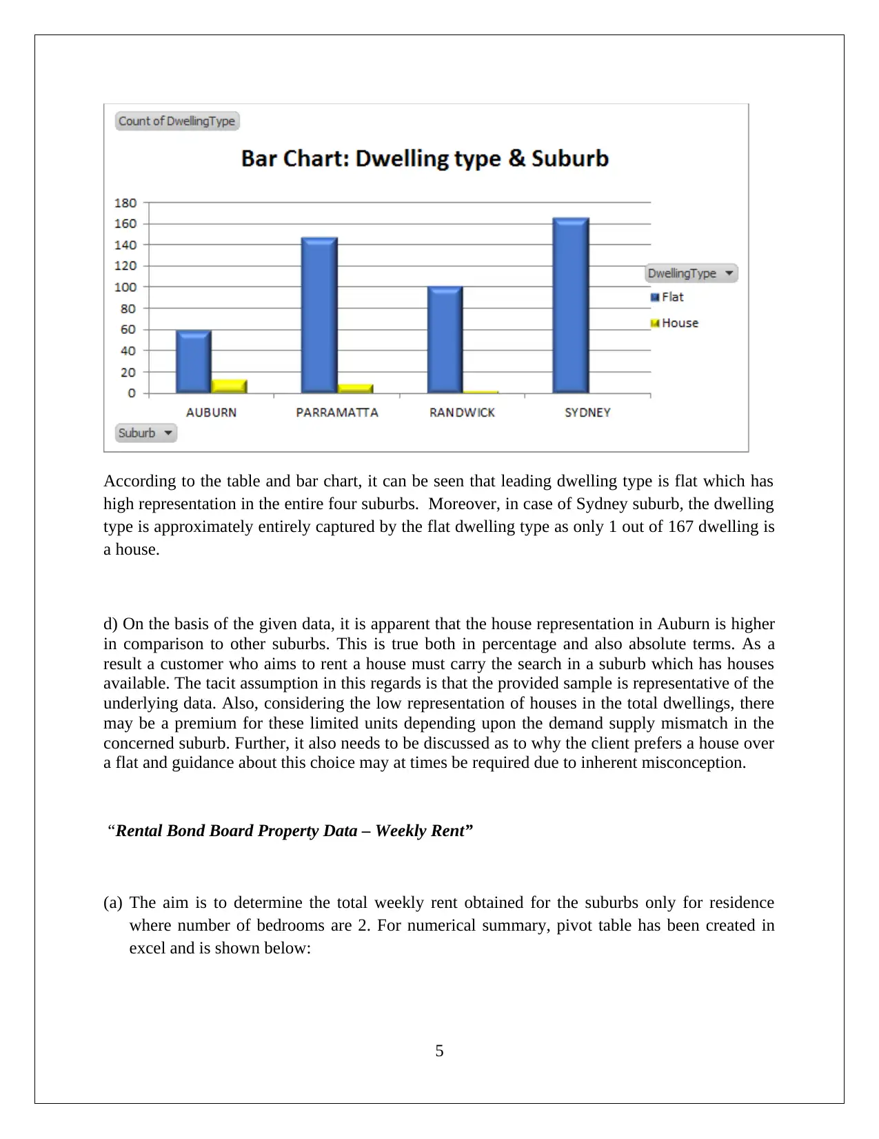
According to the table and bar chart, it can be seen that leading dwelling type is flat which has
high representation in the entire four suburbs. Moreover, in case of Sydney suburb, the dwelling
type is approximately entirely captured by the flat dwelling type as only 1 out of 167 dwelling is
a house.
d) On the basis of the given data, it is apparent that the house representation in Auburn is higher
in comparison to other suburbs. This is true both in percentage and also absolute terms. As a
result a customer who aims to rent a house must carry the search in a suburb which has houses
available. The tacit assumption in this regards is that the provided sample is representative of the
underlying data. Also, considering the low representation of houses in the total dwellings, there
may be a premium for these limited units depending upon the demand supply mismatch in the
concerned suburb. Further, it also needs to be discussed as to why the client prefers a house over
a flat and guidance about this choice may at times be required due to inherent misconception.
“Rental Bond Board Property Data – Weekly Rent”
(a) The aim is to determine the total weekly rent obtained for the suburbs only for residence
where number of bedrooms are 2. For numerical summary, pivot table has been created in
excel and is shown below:
5

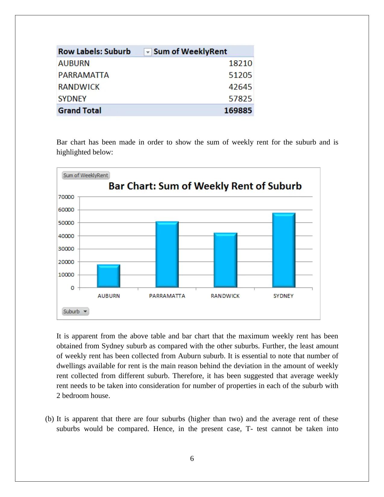
Bar chart has been made in order to show the sum of weekly rent for the suburb and is
highlighted below:
It is apparent from the above table and bar chart that the maximum weekly rent has been
obtained from Sydney suburb as compared with the other suburbs. Further, the least amount
of weekly rent has been collected from Auburn suburb. It is essential to note that number of
dwellings available for rent is the main reason behind the deviation in the amount of weekly
rent collected from different suburb. Therefore, it has been suggested that average weekly
rent needs to be taken into consideration for number of properties in each of the suburb with
2 bedroom house.
(b) It is apparent that there are four suburbs (higher than two) and the average rent of these
suburbs would be compared. Hence, in the present case, T- test cannot be taken into
6

consideration and hence, ANOVA single test would be used. This is because ANOVA test
would provide the comparison between the weekly rents for the given suburbs.
Null hypothesis H0 :The mean weekly rent of the dwellings in all the suburbs is same.
Alternative hypothesis H1 : The mean weekly rent of dwellings in atleast one suburb is different
from the other suburbs
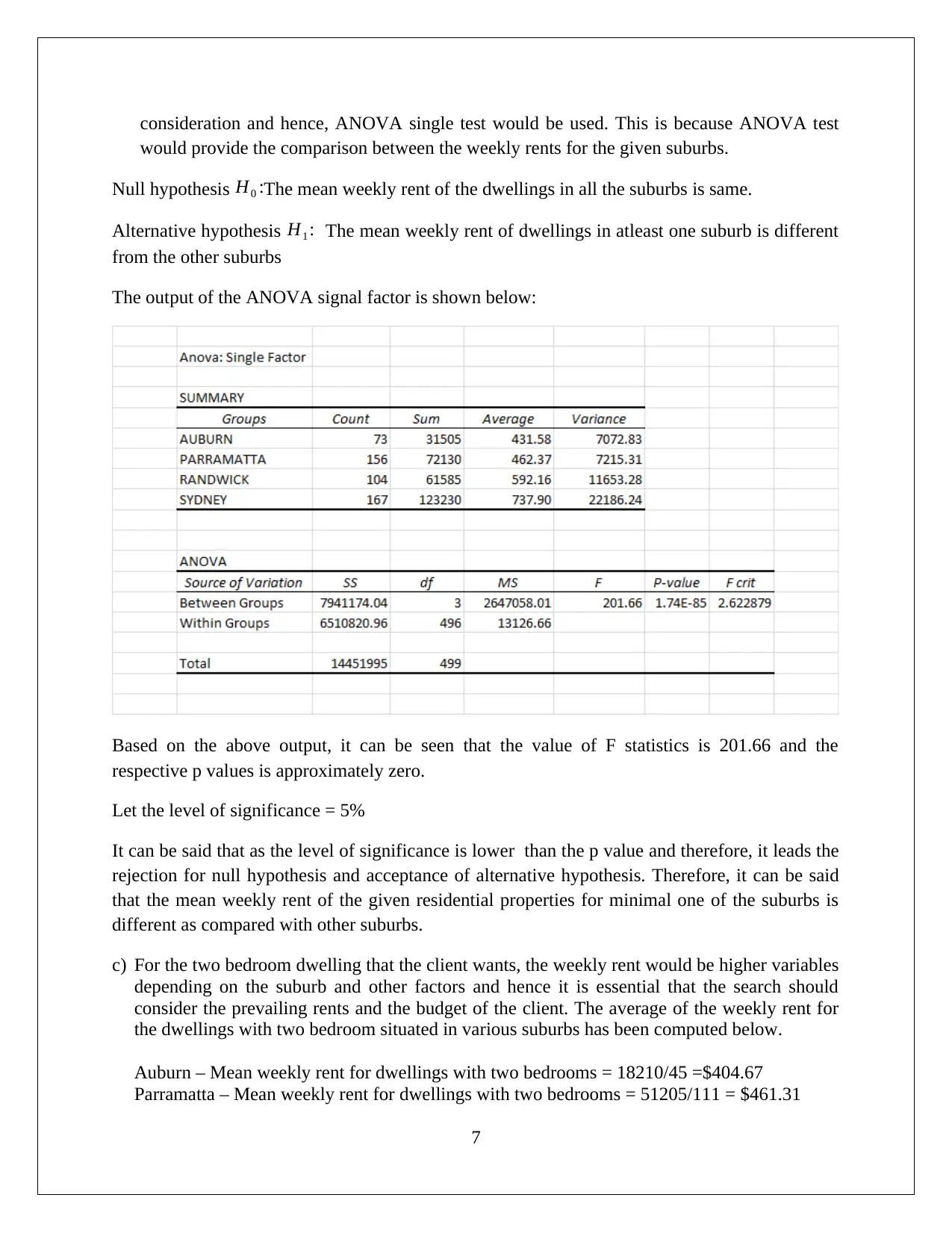
The output of the ANOVA signal factor is shown below:
Based on the above output, it can be seen that the value of F statistics is 201.66 and the
respective p values is approximately zero.
Let the level of significance = 5%
It can be said that as the level of significance is lower than the p value and therefore, it leads the
rejection for null hypothesis and acceptance of alternative hypothesis. Therefore, it can be said
that the mean weekly rent of the given residential properties for minimal one of the suburbs is
different as compared with other suburbs.
c) For the two bedroom dwelling that the client wants, the weekly rent would be higher variables
depending on the suburb and other factors and hence it is essential that the search should
consider the prevailing rents and the budget of the client. The average of the weekly rent for
the dwellings with two bedroom situated in various suburbs has been computed below.
Auburn – Mean weekly rent for dwellings with two bedrooms = 18210/45 =$404.67
Parramatta – Mean weekly rent for dwellings with two bedrooms = 51205/111 = $461.31
7

Randwick – Mean weekly rent for dwellings with two bedrooms = 42645/69 = $618
Sydney– Mean weekly rent for dwellings with two bedrooms = 57825/69 = $838.04
From the above calculation, it would be fair to infer that rent for a dwelling wih 2 bedroom is
the cheapest in Auburn and most expensive in Sydney. Thus, based on the available budget
only should the client narrow down on suburbs.
Bond Amount
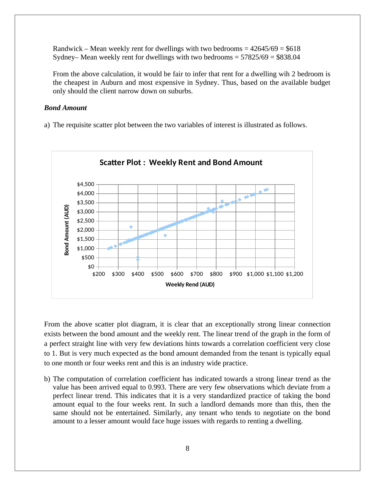
a) The requisite scatter plot between the two variables of interest is illustrated as follows.
From the above scatter plot diagram, it is clear that an exceptionally strong linear connection
exists between the bond amount and the weekly rent. The linear trend of the graph in the form of
a perfect straight line with very few deviations hints towards a correlation coefficient very close
to 1. But is very much expected as the bond amount demanded from the tenant is typically equal
to one month or four weeks rent and this is an industry wide practice.
b) The computation of correlation coefficient has indicated towards a strong linear trend as the
value has been arrived equal to 0.993. There are very few observations which deviate from a
perfect linear trend. This indicates that it is a very standardized practice of taking the bond
amount equal to the four weeks rent. In such a landlord demands more than this, then the
same should not be entertained. Similarly, any tenant who tends to negotiate on the bond
amount to a lesser amount would face huge issues with regards to renting a dwelling.
8
$200 $300 $400 $500 $600 $700 $800 $900 $1,000 $1,100 $1,200
$0
$500
$1,000
$1,500
$2,000
$2,500
$3,000
$3,500
$4,000
$4,500
Scatter Plot : Weekly Rent and Bond Amount
Weekly Rend (AUD)
Bond Amount (AUD)

Conclusion
a) On the basis of the descriptive statistical analysis of the weekly rent of the international
students, it is apparent that the relevant data has presence of skew which leads to the
conclusion that the distribution is not normal. Even though there is low variation in the data
but the suitable average value would be captured by median owing to outlier being present. In
relation to the selected suburb data, it is apparent that the availability of flats seems to be
significantly higher in comparison with houses. Also, the client needs to be mindful of the
fact that house availability is not the same in each suburb and hence plan the search
accordingly. Also, taking into consideration the provided sample rent data, it has been
inferred that the rent across suburbs tends to differ. Further, the relationship between the bond
amount and the weekly rent is linear and quite strong which is on expected lines as the bond
amount is expressed in terms of weekly rent only.
b) In regards to future research, rather than limiting to dwelling type, other attributes such as
bedrooms should be considered so as to make out the trends followed by various suburbs and the
key similarities and differences. This would allow the clients to understand the suburbs that are
comparatively cheaper and thereby ensure higher satisfaction level from the choice of house
while ensuring that budgets are not breached. Further, based on the bedroom and other key
attributes this exercise can be carried out so as to uncover hidden price anomalies.
9