Business Analysis: Pfeiffer Company, Hartmann Portfolio Optimization
VerifiedAdded on 2023/01/20
|13
|2716
|32
Homework Assignment
AI Summary
This assignment analyzes the Hartmann portfolio managed by the Pfeiffer Company, focusing on investment optimization and risk management. The student develops and applies linear programming models to determine the optimal allocation of investments across growth stock, income, and money market funds, considering constraints such as minimum investment percentages and the client's risk tolerance. The analysis includes sensitivity analysis to assess the impact of changes in forecasted yields and risk tolerance on portfolio performance. The student also explores scenarios involving overtime and revised yield estimates, providing recommendations for portfolio revisions and automated management. Furthermore, the assignment covers decision-making models for buy/sell decisions in the context of fluctuating market prices to maximize profits over a specific period, incorporating constraints like battery capacity and end-of-period stock levels.

Business Analysis
Student Name
Institution Name
Date
1
Student Name
Institution Name
Date
1
Paraphrase This Document
Need a fresh take? Get an instant paraphrase of this document with our AI Paraphraser
Chapter 8
Problem 28
The Pfeiffer company investment management
a) Development of a liner programming model
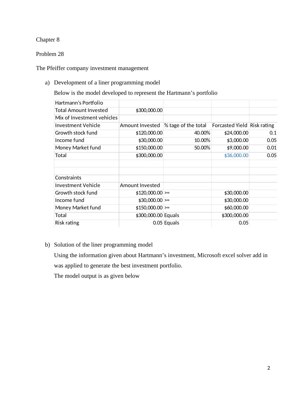
Below is the model developed to represent the Hartmann’s portfolio
Hartmann's Portfolio
Total Amount Invested $300,000.00
Mix of Investment vehicles
Investment Vehicle Amount Invested % tage of the total Forcasted Yield Risk rating
Growth stock fund $120,000.00 40.00% $24,000.00 0.1
Income fund $30,000.00 10.00% $3,000.00 0.05
Money Market fund $150,000.00 50.00% $9,000.00 0.01
Total $300,000.00 $36,000.00 0.05
Constraints
Investment Vehicle Amount Invested
Growth stock fund $120,000.00 >= $30,000.00
Income fund $30,000.00 >= $30,000.00
Money Market fund $150,000.00 >= $60,000.00
Total $300,000.00 Equals $300,000.00
Risk rating 0.05 Equals 0.05
b) Solution of the liner programming model
Using the information given about Hartmann’s investment, Microsoft excel solver add in
was applied to generate the best investment portfolio.
The model output is as given below
2
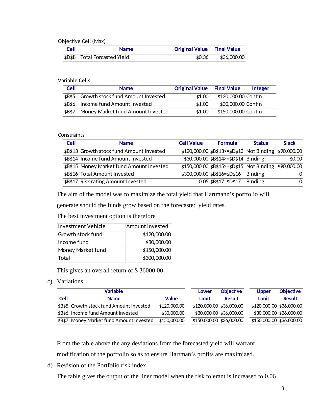
Objective Cell (Max)
Cell Name Original Value Final Value
$D$8 Total Forcasted Yield $0.36 $36,000.00
Variable Cells
Cell Name Original Value Final Value Integer
$B$5 Growth stock fund Amount Invested $1.00 $120,000.00 Contin
$B$6 Income fund Amount Invested $1.00 $30,000.00 Contin
$B$7 Money Market fund Amount Invested $1.00 $150,000.00 Contin
Constraints
Cell Name Cell Value Formula Status Slack
$B$13 Growth stock fund Amount Invested $120,000.00 $B$13>=$D$13 Not Binding $90,000.00
$B$14 Income fund Amount Invested $30,000.00 $B$14>=$D$14 Binding $0.00
$B$15 Money Market fund Amount Invested $150,000.00 $B$15>=$D$15 Not Binding $90,000.00
$B$16 Total Amount Invested $300,000.00 $B$16=$D$16 Binding 0
$B$17 Risk rating Amount Invested 0.05 $B$17=$D$17 Binding 0
The aim of the model was to maximize the total yield that Hartmann’s portfolio will
generate should the funds grow based on the forecasted yield rates.
The best investment option is therefore
Investment Vehicle Amount Invested
Growth stock fund $120,000.00
Income fund $30,000.00
Money Market fund $150,000.00
Total $300,000.00
This gives an overall return of $ 36000.00
c) Variations
Variable Lower Objective Upper Objective
Cell Name Value Limit Result Limit Result
$B$5 Growth stock fund Amount Invested $120,000.00 $120,000.00 $36,000.00 $120,000.00 $36,000.00
$B$6 Income fund Amount Invested $30,000.00 $30,000.00 $36,000.00 $30,000.00 $36,000.00
$B$7 Money Market fund Amount Invested $150,000.00 $150,000.00 $36,000.00 $150,000.00 $36,000.00
From the table above the any deviations from the forecasted yield will warrant
modification of the portfolio so as to ensure Hartman’s profits are maximized.
d) Revision of the Portfolio risk index
The table gives the output of the liner model when the risk tolerant is increased to 0.06
3
⊘ This is a preview!⊘
Do you want full access?
Subscribe today to unlock all pages.

Trusted by 1+ million students worldwide
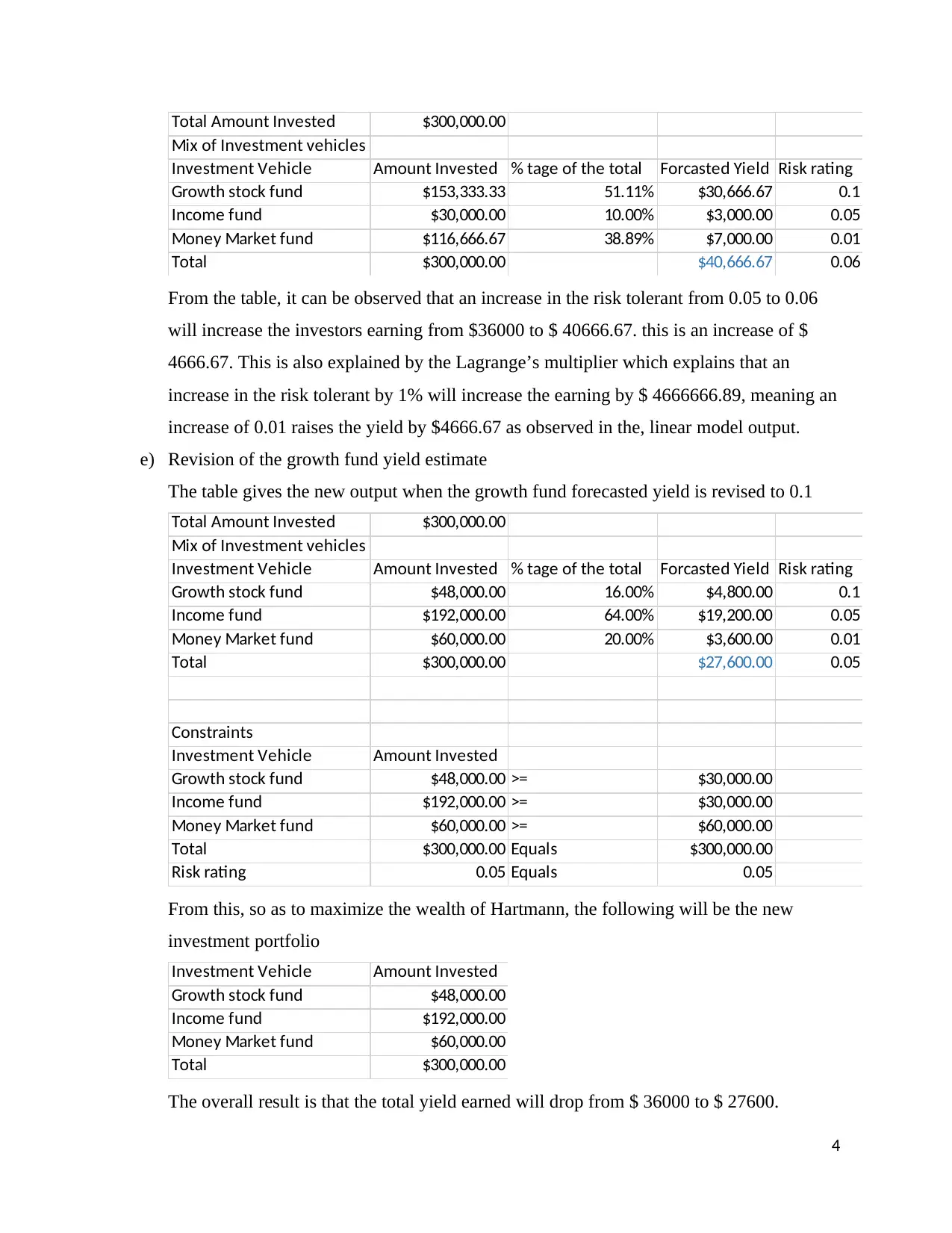
Total Amount Invested $300,000.00
Mix of Investment vehicles
Investment Vehicle Amount Invested % tage of the total Forcasted Yield Risk rating
Growth stock fund $153,333.33 51.11% $30,666.67 0.1
Income fund $30,000.00 10.00% $3,000.00 0.05
Money Market fund $116,666.67 38.89% $7,000.00 0.01
Total $300,000.00 $40,666.67 0.06
From the table, it can be observed that an increase in the risk tolerant from 0.05 to 0.06
will increase the investors earning from $36000 to $ 40666.67. this is an increase of $
4666.67. This is also explained by the Lagrange’s multiplier which explains that an
increase in the risk tolerant by 1% will increase the earning by $ 4666666.89, meaning an
increase of 0.01 raises the yield by $4666.67 as observed in the, linear model output.
e) Revision of the growth fund yield estimate
The table gives the new output when the growth fund forecasted yield is revised to 0.1
Total Amount Invested $300,000.00
Mix of Investment vehicles
Investment Vehicle Amount Invested % tage of the total Forcasted Yield Risk rating
Growth stock fund $48,000.00 16.00% $4,800.00 0.1
Income fund $192,000.00 64.00% $19,200.00 0.05
Money Market fund $60,000.00 20.00% $3,600.00 0.01
Total $300,000.00 $27,600.00 0.05
Constraints
Investment Vehicle Amount Invested
Growth stock fund $48,000.00 >= $30,000.00
Income fund $192,000.00 >= $30,000.00
Money Market fund $60,000.00 >= $60,000.00
Total $300,000.00 Equals $300,000.00
Risk rating 0.05 Equals 0.05
From this, so as to maximize the wealth of Hartmann, the following will be the new
investment portfolio
Investment Vehicle Amount Invested
Growth stock fund $48,000.00
Income fund $192,000.00
Money Market fund $60,000.00
Total $300,000.00
The overall result is that the total yield earned will drop from $ 36000 to $ 27600.
4
Mix of Investment vehicles
Investment Vehicle Amount Invested % tage of the total Forcasted Yield Risk rating
Growth stock fund $153,333.33 51.11% $30,666.67 0.1
Income fund $30,000.00 10.00% $3,000.00 0.05
Money Market fund $116,666.67 38.89% $7,000.00 0.01
Total $300,000.00 $40,666.67 0.06
From the table, it can be observed that an increase in the risk tolerant from 0.05 to 0.06
will increase the investors earning from $36000 to $ 40666.67. this is an increase of $
4666.67. This is also explained by the Lagrange’s multiplier which explains that an
increase in the risk tolerant by 1% will increase the earning by $ 4666666.89, meaning an
increase of 0.01 raises the yield by $4666.67 as observed in the, linear model output.
e) Revision of the growth fund yield estimate
The table gives the new output when the growth fund forecasted yield is revised to 0.1
Total Amount Invested $300,000.00
Mix of Investment vehicles
Investment Vehicle Amount Invested % tage of the total Forcasted Yield Risk rating
Growth stock fund $48,000.00 16.00% $4,800.00 0.1
Income fund $192,000.00 64.00% $19,200.00 0.05
Money Market fund $60,000.00 20.00% $3,600.00 0.01
Total $300,000.00 $27,600.00 0.05
Constraints
Investment Vehicle Amount Invested
Growth stock fund $48,000.00 >= $30,000.00
Income fund $192,000.00 >= $30,000.00
Money Market fund $60,000.00 >= $60,000.00
Total $300,000.00 Equals $300,000.00
Risk rating 0.05 Equals 0.05
From this, so as to maximize the wealth of Hartmann, the following will be the new
investment portfolio
Investment Vehicle Amount Invested
Growth stock fund $48,000.00
Income fund $192,000.00
Money Market fund $60,000.00
Total $300,000.00
The overall result is that the total yield earned will drop from $ 36000 to $ 27600.
4
Paraphrase This Document
Need a fresh take? Get an instant paraphrase of this document with our AI Paraphraser
f) Information
So as to utilize the model in managing the portfolio of the clients, Pfeiffer need to
maintain the client’s risk tolerant and document any changes in their behavior towards
risk. This information is necessary in calculating the portfolio risk raying which intern
affects the distribution of investment to each of the available vehicles.
g) Manual modification of 50 client’s portfolio may be expensive and time consuming for
Pfeiffer limited. It is therefore recommended that this operation be made automatic by
developing a program that can revise the portfolio once the modifications of the
forecasted yield is made. This can be done using a statistical program of choice an
example being R studio.
Chapter 9
Problem 2
a. Development and implementation of the linear model
The model developed is as shown in the table below
5
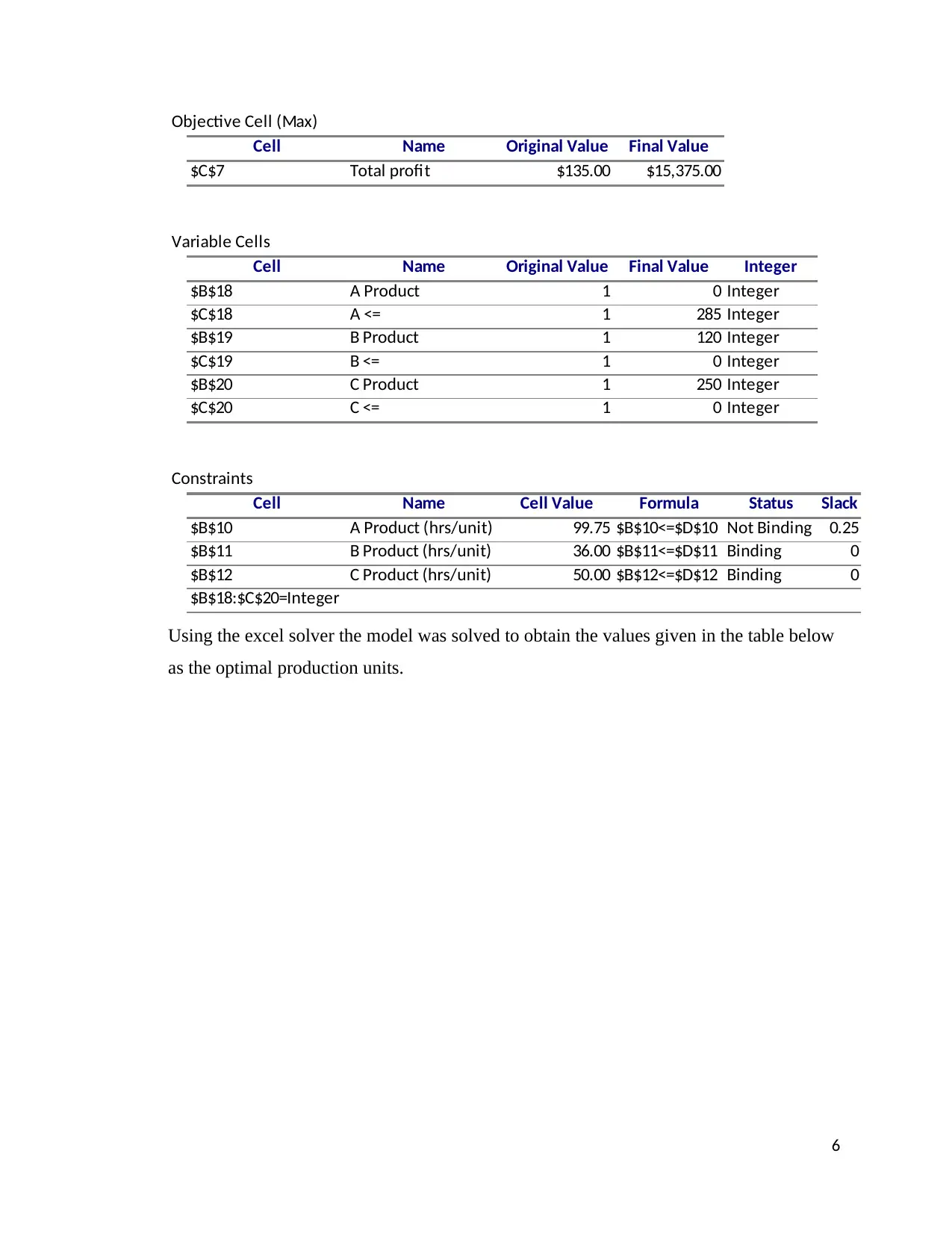
Objective Cell (Max)
Cell Name Original Value Final Value
$C$7 Total profit $135.00 $15,375.00
Variable Cells
Cell Name Original Value Final Value Integer
$B$18 A Product 1 0 Integer
$C$18 A <= 1 285 Integer
$B$19 B Product 1 120 Integer
$C$19 B <= 1 0 Integer
$B$20 C Product 1 250 Integer
$C$20 C <= 1 0 Integer
Constraints
Cell Name Cell Value Formula Status Slack
$B$10 A Product (hrs/unit) 99.75 $B$10<=$D$10 Not Binding 0.25
$B$11 B Product (hrs/unit) 36.00 $B$11<=$D$11 Binding 0
$B$12 C Product (hrs/unit) 50.00 $B$12<=$D$12 Binding 0
$B$18:$C$20=Integer
Using the excel solver the model was solved to obtain the values given in the table below
as the optimal production units.
6
⊘ This is a preview!⊘
Do you want full access?
Subscribe today to unlock all pages.

Trusted by 1+ million students worldwide
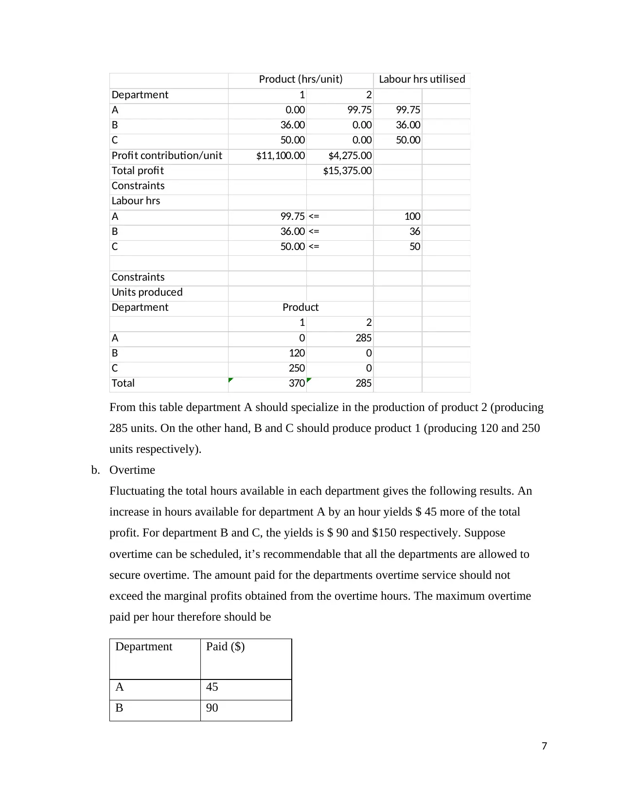
Department 1 2
A 0.00 99.75 99.75
B 36.00 0.00 36.00
C 50.00 0.00 50.00
Profit contribution/unit $11,100.00 $4,275.00
Total profit $15,375.00
Constraints
Labour hrs
A 99.75 <= 100
B 36.00 <= 36
C 50.00 <= 50
Constraints
Units produced
Department
1 2
A 0 285
B 120 0
C 250 0
Total 370 285
Product (hrs/unit) Labour hrs utilised
Product
From this table department A should specialize in the production of product 2 (producing
285 units. On the other hand, B and C should produce product 1 (producing 120 and 250
units respectively).
b. Overtime
Fluctuating the total hours available in each department gives the following results. An
increase in hours available for department A by an hour yields $ 45 more of the total
profit. For department B and C, the yields is $ 90 and $150 respectively. Suppose
overtime can be scheduled, it’s recommendable that all the departments are allowed to
secure overtime. The amount paid for the departments overtime service should not
exceed the marginal profits obtained from the overtime hours. The maximum overtime
paid per hour therefore should be
Department Paid ($)
A 45
B 90
7
Paraphrase This Document
Need a fresh take? Get an instant paraphrase of this document with our AI Paraphraser
C 150
Though the table above gives the maximum wage per hour for overtime work, the actual
amount should be lower so as to ensure the organization makes a profit from the overtime
work.
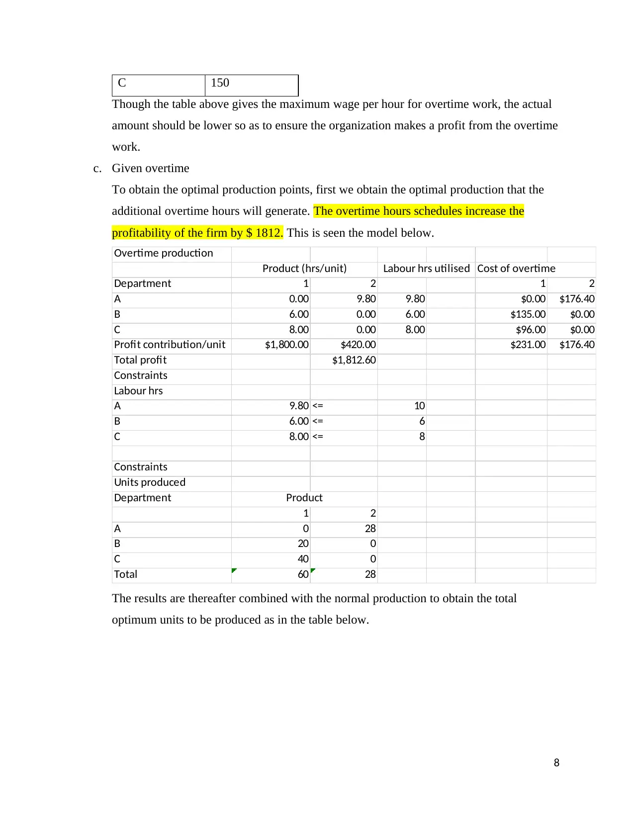
c. Given overtime
To obtain the optimal production points, first we obtain the optimal production that the
additional overtime hours will generate. The overtime hours schedules increase the
profitability of the firm by $ 1812. This is seen the model below.
Overtime production
Cost of overtime
Department 1 2 1 2
A 0.00 9.80 9.80 $0.00 $176.40
B 6.00 0.00 6.00 $135.00 $0.00
C 8.00 0.00 8.00 $96.00 $0.00
Profit contribution/unit $1,800.00 $420.00 $231.00 $176.40
Total profit $1,812.60
Constraints
Labour hrs
A 9.80 <= 10
B 6.00 <= 6
C 8.00 <= 8
Constraints
Units produced
Department
1 2
A 0 28
B 20 0
C 40 0
Total 60 28
Product (hrs/unit) Labour hrs utilised
Product
The results are thereafter combined with the normal production to obtain the total
optimum units to be produced as in the table below.
8
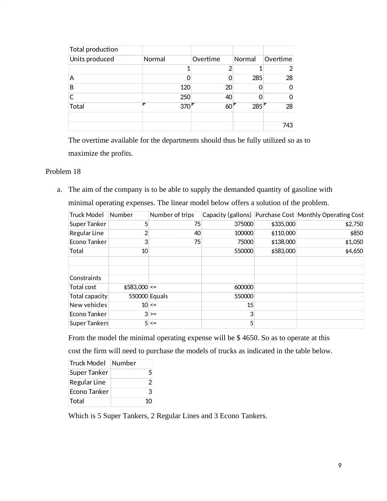
Total production
Units produced Normal Overtime Normal Overtime
1 2 1 2
A 0 0 285 28
B 120 20 0 0
C 250 40 0 0
Total 370 60 285 28
743
The overtime available for the departments should thus be fully utilized so as to
maximize the profits.
Problem 18
a. The aim of the company is to be able to supply the demanded quantity of gasoline with
minimal operating expenses. The linear model below offers a solution of the problem.
Truck Model Number Number of trips Capacity (gallons) Purchase Cost Monthly Operating Cost
Super Tanker 5 75 375000 $335,000 $2,750
Regular Line 2 40 100000 $110,000 $850
Econo Tanker 3 75 75000 $138,000 $1,050
Total 10 550000 $583,000 $4,650
Constraints
Total cost $583,000 <= 600000
Total capacity 550000 Equals 550000
New vehicles 10 <= 15
Econo Tanker 3 >= 3
Super Tankers 5 <= 5
From the model the minimal operating expense will be $ 4650. So as to operate at this
cost the firm will need to purchase the models of trucks as indicated in the table below.
Truck Model Number
Super Tanker 5
Regular Line 2
Econo Tanker 3
Total 10
Which is 5 Super Tankers, 2 Regular Lines and 3 Econo Tankers.
9
⊘ This is a preview!⊘
Do you want full access?
Subscribe today to unlock all pages.

Trusted by 1+ million students worldwide
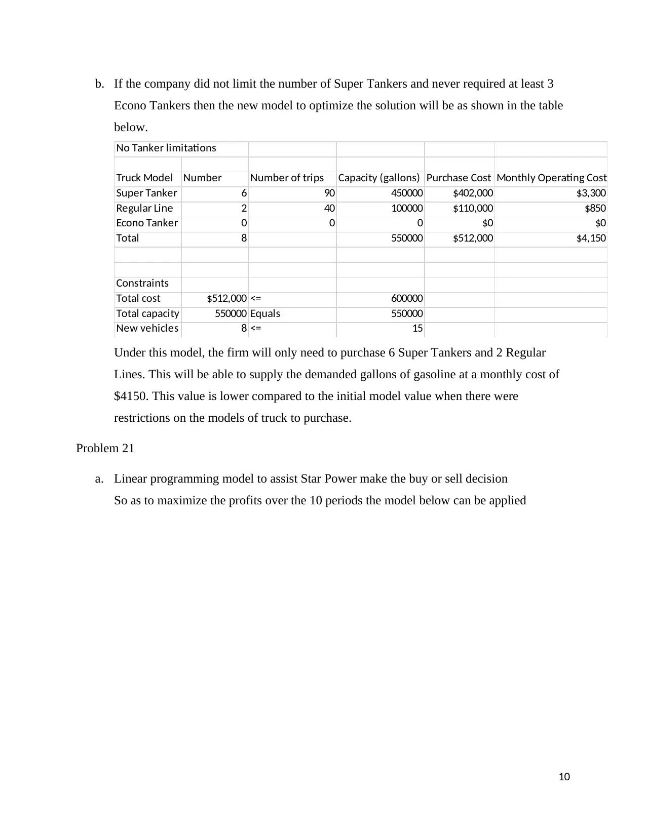
b. If the company did not limit the number of Super Tankers and never required at least 3
Econo Tankers then the new model to optimize the solution will be as shown in the table
below.
No Tanker limitations
Truck Model Number Number of trips Capacity (gallons) Purchase Cost Monthly Operating Cost
Super Tanker 6 90 450000 $402,000 $3,300
Regular Line 2 40 100000 $110,000 $850
Econo Tanker 0 0 0 $0 $0
Total 8 550000 $512,000 $4,150
Constraints
Total cost $512,000 <= 600000
Total capacity 550000 Equals 550000
New vehicles 8 <= 15
Under this model, the firm will only need to purchase 6 Super Tankers and 2 Regular
Lines. This will be able to supply the demanded gallons of gasoline at a monthly cost of
$4150. This value is lower compared to the initial model value when there were
restrictions on the models of truck to purchase.
Problem 21
a. Linear programming model to assist Star Power make the buy or sell decision
So as to maximize the profits over the 10 periods the model below can be applied
10
Paraphrase This Document
Need a fresh take? Get an instant paraphrase of this document with our AI Paraphraser
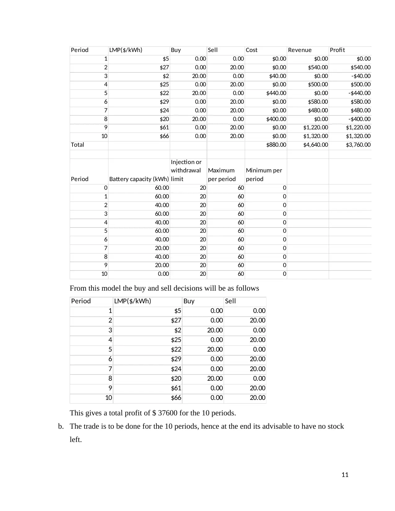
Period LMP($/kWh) Buy Sell Cost Revenue Profit
1 $5 0.00 0.00 $0.00 $0.00 $0.00
2 $27 0.00 20.00 $0.00 $540.00 $540.00
3 $2 20.00 0.00 $40.00 $0.00 -$40.00
4 $25 0.00 20.00 $0.00 $500.00 $500.00
5 $22 20.00 0.00 $440.00 $0.00 -$440.00
6 $29 0.00 20.00 $0.00 $580.00 $580.00
7 $24 0.00 20.00 $0.00 $480.00 $480.00
8 $20 20.00 0.00 $400.00 $0.00 -$400.00
9 $61 0.00 20.00 $0.00 $1,220.00 $1,220.00
10 $66 0.00 20.00 $0.00 $1,320.00 $1,320.00
Total $880.00 $4,640.00 $3,760.00
Period Battery capacity (kWh)
Injection or
withdrawal
limit
Maximum
per period
Minimum per
period
0 60.00 20 60 0
1 60.00 20 60 0
2 40.00 20 60 0
3 60.00 20 60 0
4 40.00 20 60 0
5 60.00 20 60 0
6 40.00 20 60 0
7 20.00 20 60 0
8 40.00 20 60 0
9 20.00 20 60 0
10 0.00 20 60 0
From this model the buy and sell decisions will be as follows
Period LMP($/kWh) Buy Sell
1 $5 0.00 0.00
2 $27 0.00 20.00
3 $2 20.00 0.00
4 $25 0.00 20.00
5 $22 20.00 0.00
6 $29 0.00 20.00
7 $24 0.00 20.00
8 $20 20.00 0.00
9 $61 0.00 20.00
10 $66 0.00 20.00
This gives a total profit of $ 37600 for the 10 periods.
b. The trade is to be done for the 10 periods, hence at the end its advisable to have no stock
left.
11
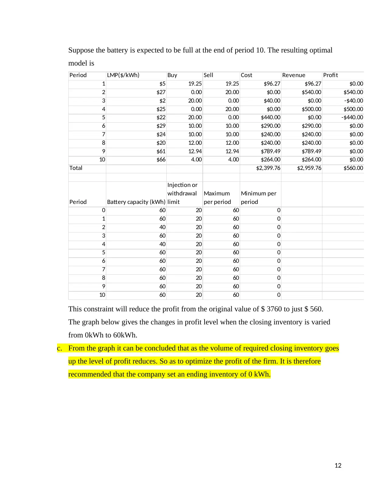
Suppose the battery is expected to be full at the end of period 10. The resulting optimal
model is
Period LMP($/kWh) Buy Sell Cost Revenue Profit
1 $5 19.25 19.25 $96.27 $96.27 $0.00
2 $27 0.00 20.00 $0.00 $540.00 $540.00
3 $2 20.00 0.00 $40.00 $0.00 -$40.00
4 $25 0.00 20.00 $0.00 $500.00 $500.00
5 $22 20.00 0.00 $440.00 $0.00 -$440.00
6 $29 10.00 10.00 $290.00 $290.00 $0.00
7 $24 10.00 10.00 $240.00 $240.00 $0.00
8 $20 12.00 12.00 $240.00 $240.00 $0.00
9 $61 12.94 12.94 $789.49 $789.49 $0.00
10 $66 4.00 4.00 $264.00 $264.00 $0.00
Total $2,399.76 $2,959.76 $560.00
Period Battery capacity (kWh)
Injection or
withdrawal
limit
Maximum
per period
Minimum per
period
0 60 20 60 0
1 60 20 60 0
2 40 20 60 0
3 60 20 60 0
4 40 20 60 0
5 60 20 60 0
6 60 20 60 0
7 60 20 60 0
8 60 20 60 0
9 60 20 60 0
10 60 20 60 0
This constraint will reduce the profit from the original value of $ 3760 to just $ 560.
The graph below gives the changes in profit level when the closing inventory is varied
from 0kWh to 60kWh.
c. From the graph it can be concluded that as the volume of required closing inventory goes
up the level of profit reduces. So as to optimize the profit of the firm. It is therefore
recommended that the company set an ending inventory of 0 kWh.
12
⊘ This is a preview!⊘
Do you want full access?
Subscribe today to unlock all pages.

Trusted by 1+ million students worldwide
1 out of 13
Your All-in-One AI-Powered Toolkit for Academic Success.
+13062052269
info@desklib.com
Available 24*7 on WhatsApp / Email
![[object Object]](/_next/static/media/star-bottom.7253800d.svg)
Unlock your academic potential
Copyright © 2020–2025 A2Z Services. All Rights Reserved. Developed and managed by ZUCOL.