Statistical Technique for Business Assignment
VerifiedAdded on 2023/04/21
|10
|2239
|365
AI Summary
This assignment discusses the use of statistical techniques for business assignments and focuses on modeling water usage. It explores the variables of temperature, production, days, and persons and their impact on water usage. The assignment also includes methods, results, model evaluation, assumptions, and a conclusion.
Contribute Materials
Your contribution can guide someone’s learning journey. Share your
documents today.
BUSINESS ANALYTICS 1
Statistical Technique for Business Assignment
Student’s Registration Number
Name of Student
Course Title
Submission Date
Statistical Technique for Business Assignment
Student’s Registration Number
Name of Student
Course Title
Submission Date
Secure Best Marks with AI Grader
Need help grading? Try our AI Grader for instant feedback on your assignments.
BUSINESS ANALYTICS 2
Table of Content
Introduction ……………………………………………………………………………4
Methods ………………………………………………………………………………...5
Results ………………………………………………………………………………….6
Model evaluation ………………………………………………………………………8
Assumption …………………………………………………………………………….8
Conclusion ……………………………………………………………………………..9
References…………………………………………………………………………….10
Appendix ……………………………………………………………………………..11
BUSINESS ANALYTICS 3
Introduction
The aim of the assignment is to model the water usage. Every company or any business aims at
minimizing the cost of production while maximizing the profit, To achieve this, the company try
to come up with options that will help maximize the profit and minimize the cost. Cost of
production is inevitable for the company and therefore, they cannot avoid it. The best way to
tackle this problem is to conduct an analysis of the possible input on the company. The data
should be collected in a systematic way in order to achieve the desired results. After the data
collection, the data is manipulated and aggregated to make the analysis simpler and easier.
Thereafter, the desired variables are chosen and the appropriate data analysis is conducted.
In our case, we have been provided with a dataset containing the following variables:
Temperature, Production, Persons, Days, Supervisor and Water. The data was obtained from a
Production plant. The main issue is the cost of production. The issue is present due to the
monthly usage which is too high. Data were collected to investigate water usage. Using the data
obtained by the production plant, a model is to be created to investigate the above objective. The
data will be manipulated so that we come up with the best model. Additionally, the desired
variables will be chosen to help model the data.

BUSINESS ANALYTICS 4
Methods
The data was modeled using multiple regressions. Just like simple linear regression, multiple
regressions use the same concepts. The only difference is that it contains more than 1
independent variable Draper and Smith (2014). The importance of multiple regressions is that it
predicts the outcome of the dependent variable using several predictor variables Keith (2014).
Multiple regressions use the concept of a mathematical equation to develop the relationship
between variables i.e. dependent and independent variables. By conducting multiple regressions,
we will be able to show the effect of the independent variables on dependent variables. We will
also be able to test whether the effect is valid or not. In our scenario, the usage of water is to be
predicted using the chosen variables. From the model, we will be able to come up with insight
and a conclusion that will help handle water usage. To create a multiple regression, we need to
come up with more than one independent variables and dependent variable. After importing the
dataset to the R studio, one needs to select the best variables to be used to create the regression
model. Variables chosen should be numbers or integers. After, the selection, the linear model
formula is created to represent the regression analysis. A name is assigned to the model and if
you use a summary function to the linear model, you will obtain the required results under
coefficient part. In our model, we will use 4 independent variables. They are Temperature,
Production, Days and Persons. The general formula for our multiple linear regressions is:
Y = 0 + 1X1 + 2X2 + 3X3+ 4X4
Where:
Y= water usage
X1 = Temperature
X2 = Production (Cost of Production)
Secure Best Marks with AI Grader
Need help grading? Try our AI Grader for instant feedback on your assignments.
BUSINESS ANALYTICS 5
X3 = Days (Number of days)
X4 = Persons (Total number of people)
0 = y-intercept
1, 2, 2, 3 and 4 = coefficient estimates
The dependent variable was transformed using logarithm before conducting the regression
analysis in order to achieve a normal distribution model.
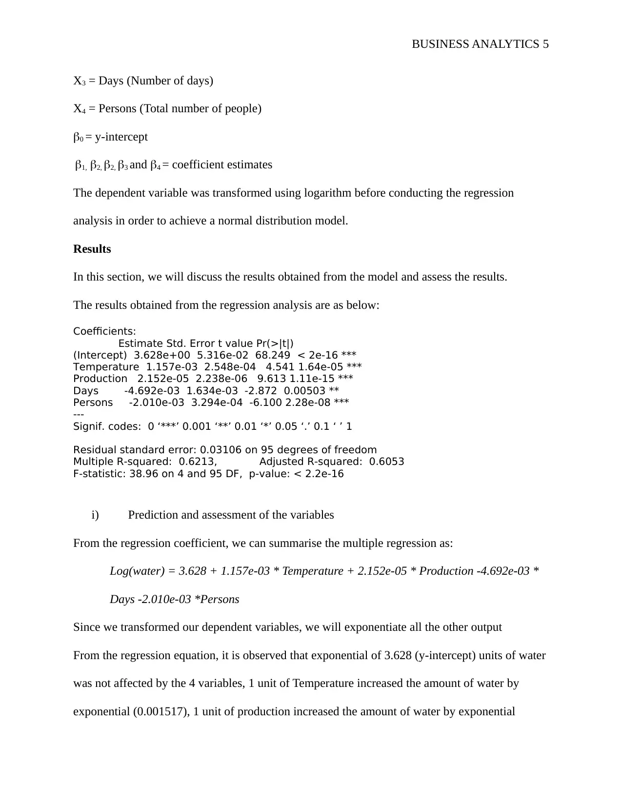
Results
In this section, we will discuss the results obtained from the model and assess the results.
The results obtained from the regression analysis are as below:
Coefficients:
Estimate Std. Error t value Pr(>|t|)
(Intercept) 3.628e+00 5.316e-02 68.249 < 2e-16 ***
Temperature 1.157e-03 2.548e-04 4.541 1.64e-05 ***
Production 2.152e-05 2.238e-06 9.613 1.11e-15 ***
Days -4.692e-03 1.634e-03 -2.872 0.00503 **
Persons -2.010e-03 3.294e-04 -6.100 2.28e-08 ***
---
Signif. codes: 0 ‘***’ 0.001 ‘**’ 0.01 ‘*’ 0.05 ‘.’ 0.1 ‘ ’ 1
Residual standard error: 0.03106 on 95 degrees of freedom
Multiple R-squared: 0.6213, Adjusted R-squared: 0.6053
F-statistic: 38.96 on 4 and 95 DF, p-value: < 2.2e-16
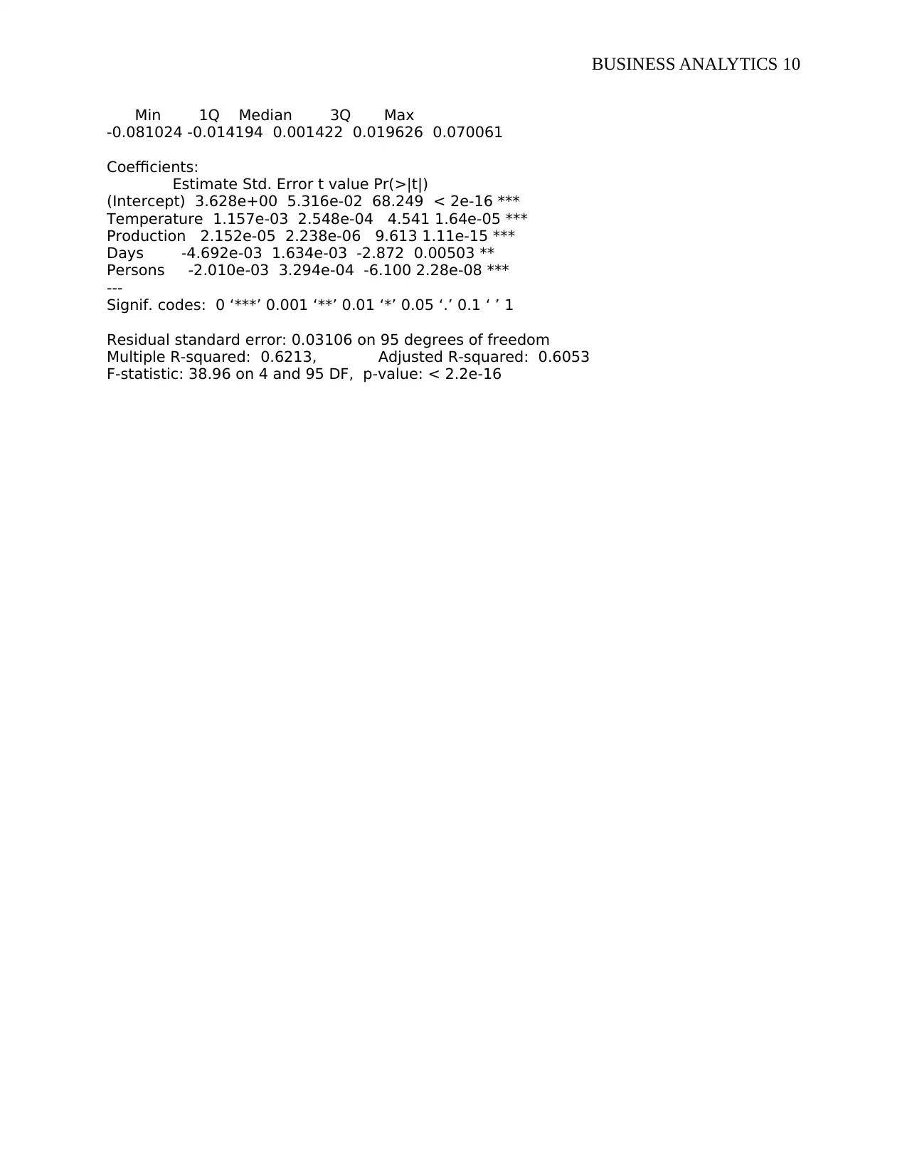
i) Prediction and assessment of the variables
From the regression coefficient, we can summarise the multiple regression as:
Log(water) = 3.628 + 1.157e-03 * Temperature + 2.152e-05 * Production -4.692e-03 *
Days -2.010e-03 *Persons
Since we transformed our dependent variables, we will exponentiate all the other output
From the regression equation, it is observed that exponential of 3.628 (y-intercept) units of water
was not affected by the 4 variables, 1 unit of Temperature increased the amount of water by
exponential (0.001517), 1 unit of production increased the amount of water by exponential
X3 = Days (Number of days)
X4 = Persons (Total number of people)
0 = y-intercept
1, 2, 2, 3 and 4 = coefficient estimates
The dependent variable was transformed using logarithm before conducting the regression
analysis in order to achieve a normal distribution model.
Results
In this section, we will discuss the results obtained from the model and assess the results.
The results obtained from the regression analysis are as below:
Coefficients:
Estimate Std. Error t value Pr(>|t|)
(Intercept) 3.628e+00 5.316e-02 68.249 < 2e-16 ***
Temperature 1.157e-03 2.548e-04 4.541 1.64e-05 ***
Production 2.152e-05 2.238e-06 9.613 1.11e-15 ***
Days -4.692e-03 1.634e-03 -2.872 0.00503 **
Persons -2.010e-03 3.294e-04 -6.100 2.28e-08 ***
---
Signif. codes: 0 ‘***’ 0.001 ‘**’ 0.01 ‘*’ 0.05 ‘.’ 0.1 ‘ ’ 1
Residual standard error: 0.03106 on 95 degrees of freedom
Multiple R-squared: 0.6213, Adjusted R-squared: 0.6053
F-statistic: 38.96 on 4 and 95 DF, p-value: < 2.2e-16
i) Prediction and assessment of the variables
From the regression coefficient, we can summarise the multiple regression as:
Log(water) = 3.628 + 1.157e-03 * Temperature + 2.152e-05 * Production -4.692e-03 *
Days -2.010e-03 *Persons
Since we transformed our dependent variables, we will exponentiate all the other output
From the regression equation, it is observed that exponential of 3.628 (y-intercept) units of water
was not affected by the 4 variables, 1 unit of Temperature increased the amount of water by
exponential (0.001517), 1 unit of production increased the amount of water by exponential
BUSINESS ANALYTICS 6
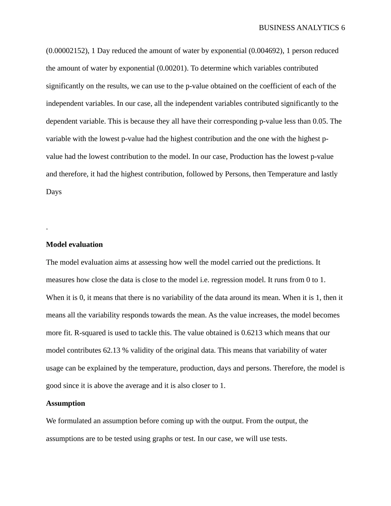
(0.00002152), 1 Day reduced the amount of water by exponential (0.004692), 1 person reduced
the amount of water by exponential (0.00201). To determine which variables contributed
significantly on the results, we can use to the p-value obtained on the coefficient of each of the
independent variables. In our case, all the independent variables contributed significantly to the
dependent variable. This is because they all have their corresponding p-value less than 0.05. The
variable with the lowest p-value had the highest contribution and the one with the highest p-
value had the lowest contribution to the model. In our case, Production has the lowest p-value
and therefore, it had the highest contribution, followed by Persons, then Temperature and lastly
Days
.
Model evaluation
The model evaluation aims at assessing how well the model carried out the predictions. It
measures how close the data is close to the model i.e. regression model. It runs from 0 to 1.
When it is 0, it means that there is no variability of the data around its mean. When it is 1, then it
means all the variability responds towards the mean. As the value increases, the model becomes
more fit. R-squared is used to tackle this. The value obtained is 0.6213 which means that our
model contributes 62.13 % validity of the original data. This means that variability of water
usage can be explained by the temperature, production, days and persons. Therefore, the model is
good since it is above the average and it is also closer to 1.
Assumption
We formulated an assumption before coming up with the output. From the output, the
assumptions are to be tested using graphs or test. In our case, we will use tests.
BUSINESS ANALYTICS 7
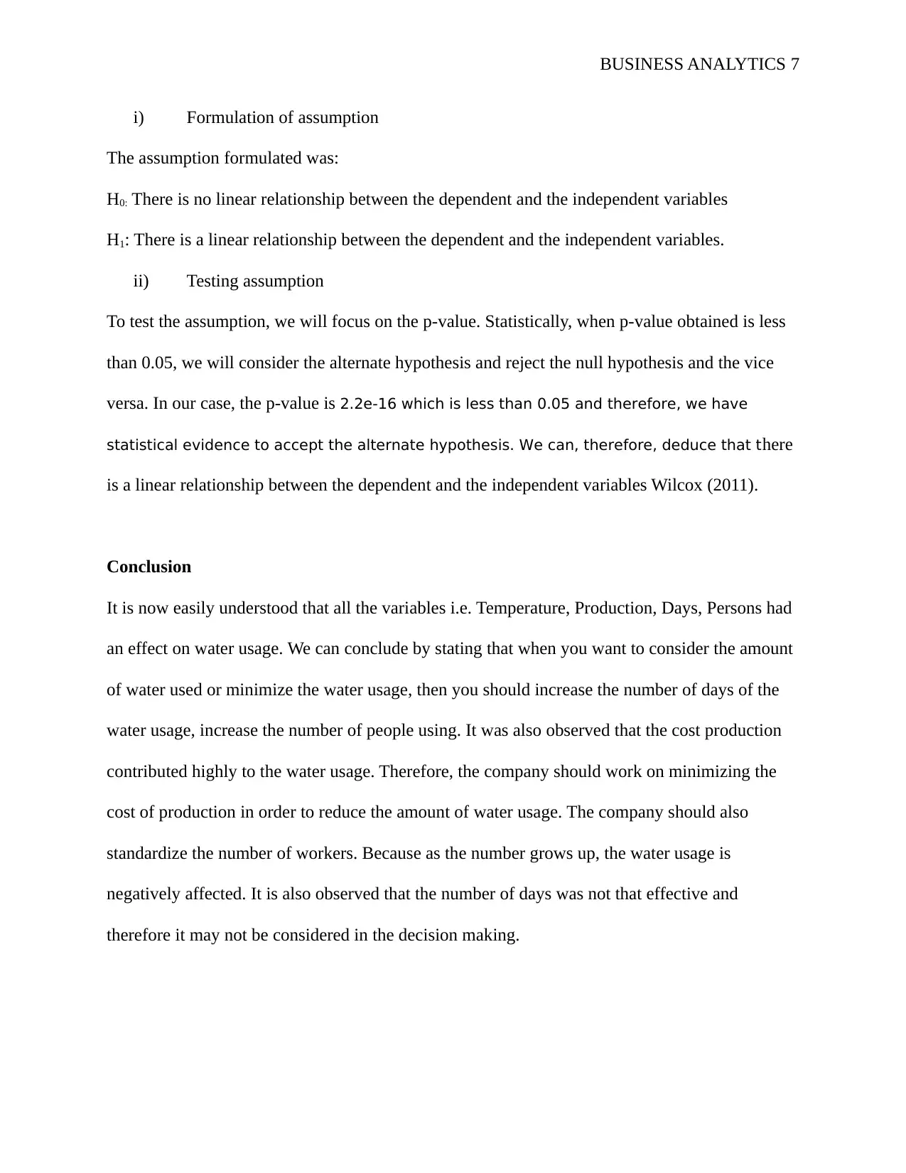
i) Formulation of assumption
The assumption formulated was:
H0: There is no linear relationship between the dependent and the independent variables
H1: There is a linear relationship between the dependent and the independent variables.
ii) Testing assumption
To test the assumption, we will focus on the p-value. Statistically, when p-value obtained is less
than 0.05, we will consider the alternate hypothesis and reject the null hypothesis and the vice
versa. In our case, the p-value is 2.2e-16 which is less than 0.05 and therefore, we have
statistical evidence to accept the alternate hypothesis. We can, therefore, deduce that there
is a linear relationship between the dependent and the independent variables Wilcox (2011).
Conclusion
It is now easily understood that all the variables i.e. Temperature, Production, Days, Persons had
an effect on water usage. We can conclude by stating that when you want to consider the amount
of water used or minimize the water usage, then you should increase the number of days of the
water usage, increase the number of people using. It was also observed that the cost production
contributed highly to the water usage. Therefore, the company should work on minimizing the
cost of production in order to reduce the amount of water usage. The company should also
standardize the number of workers. Because as the number grows up, the water usage is
negatively affected. It is also observed that the number of days was not that effective and
therefore it may not be considered in the decision making.
Paraphrase This Document
Need a fresh take? Get an instant paraphrase of this document with our AI Paraphraser
BUSINESS ANALYTICS 8
References
Draper, N.R. and Smith, H., 2014. Applied regression analysis (Vol. 326). John Wiley & Sons.
Keith, T.Z., 2014. Multiple regression and beyond: An introduction to multiple regression and
structural equation modeling.New York: Routledge.
Wilcox, R.R., 2011. Introduction to robust estimation and hypothesis testing. 3 rd ed.
Cambridge:Academic press
BUSINESS ANALYTICS 9
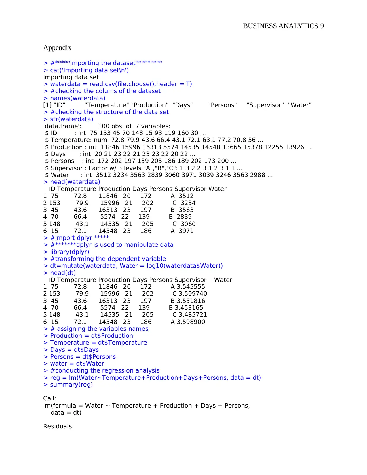
Appendix
> #*****importing the dataset*********
> cat('Importing data set\n')
Importing data set
> waterdata = read.csv(file.choose(),header = T)
> #checking the colums of the dataset
> names(waterdata)
[1] "ID" "Temperature" "Production" "Days" "Persons" "Supervisor" "Water"
> #checking the structure of the data set
> str(waterdata)
'data.frame': 100 obs. of 7 variables:
$ ID : int 75 153 45 70 148 15 93 119 160 30 ...
$ Temperature: num 72.8 79.9 43.6 66.4 43.1 72.1 63.1 77.2 70.8 56 ...
$ Production : int 11846 15996 16313 5574 14535 14548 13665 15378 12255 13926 ...
$ Days : int 20 21 23 22 21 23 23 22 20 22 ...
$ Persons : int 172 202 197 139 205 186 189 202 173 200 ...
$ Supervisor : Factor w/ 3 levels "A","B","C": 1 3 2 2 3 1 2 3 1 1 ...
$ Water : int 3512 3234 3563 2839 3060 3971 3039 3246 3563 2988 ...
> head(waterdata)
ID Temperature Production Days Persons Supervisor Water
1 75 72.8 11846 20 172 A 3512
2 153 79.9 15996 21 202 C 3234
3 45 43.6 16313 23 197 B 3563
4 70 66.4 5574 22 139 B 2839
5 148 43.1 14535 21 205 C 3060
6 15 72.1 14548 23 186 A 3971
> #import dplyr *****
> #*******dplyr is used to manipulate data
> library(dplyr)
> #transforming the dependent variable
> dt=mutate(waterdata, Water = log10(waterdata$Water))
> head(dt)
ID Temperature Production Days Persons Supervisor Water
1 75 72.8 11846 20 172 A 3.545555
2 153 79.9 15996 21 202 C 3.509740
3 45 43.6 16313 23 197 B 3.551816
4 70 66.4 5574 22 139 B 3.453165
5 148 43.1 14535 21 205 C 3.485721
6 15 72.1 14548 23 186 A 3.598900
> # assigning the variables names
> Production = dt$Production
> Temperature = dt$Temperature
> Days = dt$Days
> Persons = dt$Persons
> water = dt$Water
> #conducting the regression analysis
> reg = lm(Water~Temperature+Production+Days+Persons, data = dt)
> summary(reg)
Call:
lm(formula = Water ~ Temperature + Production + Days + Persons,
data = dt)
Residuals:
BUSINESS ANALYTICS 10
Min 1Q Median 3Q Max
-0.081024 -0.014194 0.001422 0.019626 0.070061
Coefficients:
Estimate Std. Error t value Pr(>|t|)
(Intercept) 3.628e+00 5.316e-02 68.249 < 2e-16 ***
Temperature 1.157e-03 2.548e-04 4.541 1.64e-05 ***
Production 2.152e-05 2.238e-06 9.613 1.11e-15 ***
Days -4.692e-03 1.634e-03 -2.872 0.00503 **
Persons -2.010e-03 3.294e-04 -6.100 2.28e-08 ***
---
Signif. codes: 0 ‘***’ 0.001 ‘**’ 0.01 ‘*’ 0.05 ‘.’ 0.1 ‘ ’ 1
Residual standard error: 0.03106 on 95 degrees of freedom
Multiple R-squared: 0.6213, Adjusted R-squared: 0.6053
F-statistic: 38.96 on 4 and 95 DF, p-value: < 2.2e-16
1 out of 10
Related Documents


Your All-in-One AI-Powered Toolkit for Academic Success.
+13062052269
info@desklib.com
Available 24*7 on WhatsApp / Email
![[object Object]](/_next/static/media/star-bottom.7253800d.svg)
Unlock your academic potential
© 2024 | Zucol Services PVT LTD | All rights reserved.