Business Analytics Assessment 1: Solutions, Analysis, and Discussion
VerifiedAdded on 2023/06/04
|17
|3851
|143
Homework Assignment
AI Summary
This document presents a comprehensive solution to Business Analytics Assessment 1, addressing key concepts in data analysis and modeling. The assessment covers topics such as handling imbalanced data in classification, the application of logistic regression, and the use of KNN models. The solution provides detailed explanations and examples of how to apply these techniques in a business context. Furthermore, the assessment explores multiple linear regression and data visualization techniques. The document includes answers to specific questions, analysis of data, and the interpretation of results, offering a thorough understanding of the subject matter. The student's work demonstrates a solid grasp of the principles and practical application of business analytics in various scenarios, from employee attendance to product yield and blood type analysis.
BUSINESS ANALYTICS: ASSESSMENT
1
BUSINESS ANALYTICS: ASSESSMENT QUESTIONS
By (Name)
The Name of the Class (Course)
Professor (Tutor)
The Name of the School (University)
The City and State where it is located
The Date
1
BUSINESS ANALYTICS: ASSESSMENT QUESTIONS
By (Name)
The Name of the Class (Course)
Professor (Tutor)
The Name of the School (University)
The City and State where it is located
The Date
Paraphrase This Document
Need a fresh take? Get an instant paraphrase of this document with our AI Paraphraser
BUSINESS ANALYTICS: ASSESSMENT
2
Business Analytics: Assessment Questions
Question 1
Imbalance data is a common problem in classification; it is created when classes are not
of equal size/ volume (Hilbe 2009). One example, the daily attendance register for employees in
an office setting, you can get that out of 200 individuals 4 were absent and 196 were present on
18th of March 2018. Another example is there are four departments (A, B, C, and D) that
generate the same product for an organization. According to data statistics collected by the
organization the overall product yield can be attributed 50% to A, 20% to B, 12% to C, and 18%
to D. These two examples show how common the issue of imbalance data is in the world of
business. To address this problem there are two techniques we can employ such as random
under-sampling and re-sampling. Random under-sampling seeks to achieve equality in class
distribution by through the random negation of the majority class. While, re-sampling technique
calls for the increment of the minority classes or an alternative would be to decrease the majority
classes in order to balance the classes (Hilbe 2009).
Question 2
In a logistic regression it is impossible to get a single line that goes through all the point
thereby indicating the line of best fit. Since, it is impossible to get the value of 1 for R squared
there is no use of R-squared and adjusted R-squared in a regression analysis. As such, special
tests have been developed to tackle this problem; for example, McFadden's pseudo-R-squared
(Hilbe 2009).
Question 3
Logistic regression can be used by business management because they can assign values
of 0s and 1s to data to distinguish the classes. For example, management can use 1s to denote
BUSINESS ANALYTICS: ASSESSMENT
3
employs who attended a meeting and 0s to indicate those who were absent from the meeting.
Another example of where logistic regression can be applied in a business setting is when
information is being collected on how many employees received bonuses. The individuals that
received bonuses will be denoted by 1s and those who did not get bonuses will be represented by
0s. Therefore, logistic regression is used in organization to analysis qualitative data with fixed
responses/choices that can be assigned numerical value.
Question 4
Each of the levels of the first explanatory variable (X1) will be assigned numerical values
that are unique. For example, 0 for low, 1 for average, 2 for high, and 3 for very high. Likewise,
the same will be done for the second explanatory variable (X2); As such, the levels will be
assigned values like 0=Sydney, 1=Melbourne, and 2=Brisbane. It is easy to see that the same
number allocation system can be used on different variables with unrelated data; given X1 deals
with a ranking system and X2 deals with Australian cities. Since we have two independent
variables where will be three coefficients i.e. B0, B1, and B2. It is important to indicate that B1
and B2 are the coefficients for X1 and X2 respectively.
Question 5
Part (a)
KNN models are based on a non-parametric learning technique through which we attempt
to predict the value of give variable based on a training set. The first step involves the evaluation
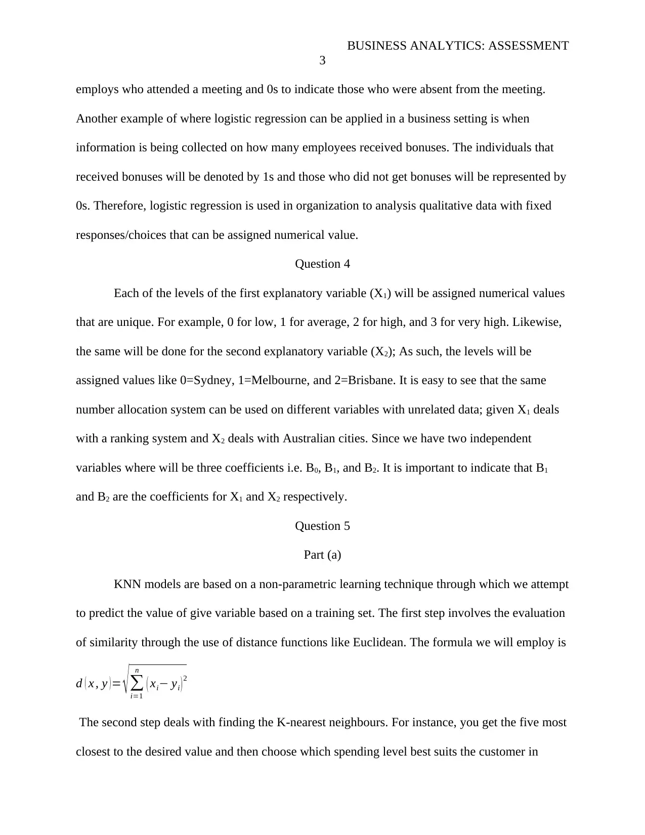
of similarity through the use of distance functions like Euclidean. The formula we will employ is
d ( x , y )= √∑
i=1
n
( xi− yi ) 2
The second step deals with finding the K-nearest neighbours. For instance, you get the five most
closest to the desired value and then choose which spending level best suits the customer in
⊘ This is a preview!⊘
Do you want full access?
Subscribe today to unlock all pages.

Trusted by 1+ million students worldwide
BUSINESS ANALYTICS: ASSESSMENT
4
question. We can also chart a graph to demonstrate the distance values to best see which ones are
closest to that of the new customer.
Part (b)
Yes, it will increase because we will be given a wide scope from where to choose the
new customers spending. Moreover, using the CONTIF function in Microsoft Excel it is clear
that 100% of all customers in the data spent more than $500; As such, it is very likely that this
new customer will spend at least $500.
Part (c)
The type of product being purchased information is omitted as such that first column will
be ignore in our calculation. After calculation the new female customer had a distance of 0 with a
pre-exist customer. Therefore, we will conclude the customer is most likely to spend $938
Question 6
Part (a)
The best thing would be to analysis the data and compare the variables to discern their
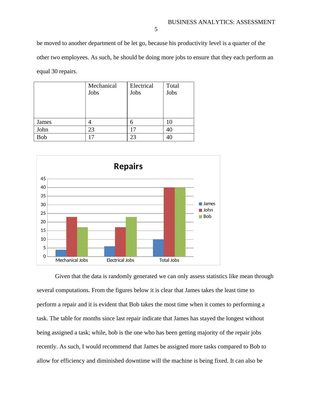
relationship. For instance, we can compare how much of a give type of repair was performed by
a particular repair person. According to the data and chart below it is clear that majority of the
repairs were done by Bob and John. Majority of the Mechanical repair jobs were performed by
John; As such, if there are constant mechanical issues being witnesses with machines the bulk of
the blame should be directed at John. It is therefore important for management to develop a plan
that will ensure that John is assessed and trained on his competence as a mechanical repair. On
the other hand, majority of the electrical repairs were performed by Bob; likewise, he should be
held as most accountable for repetitive electrical issues with the machines. It is important to note
that James has done very little compared to the other two employees. It is recommendable that he
Paraphrase This Document
Need a fresh take? Get an instant paraphrase of this document with our AI Paraphraser
BUSINESS ANALYTICS: ASSESSMENT
5
be moved to another department of be let go, because his productivity level is a quarter of the
other two employees. As such, he should be doing more jobs to ensure that they each perform an
equal 30 repairs.
Mechanical
Jobs
Electrical
Jobs
Total
Jobs
James 4 6 10
John 23 17 40
Bob 17 23 40
Mechanical Jobs Electrical Jobs Total Jobs
0
5
10
15
20
25
30
35
40
45
Repairs
James
John
Bob
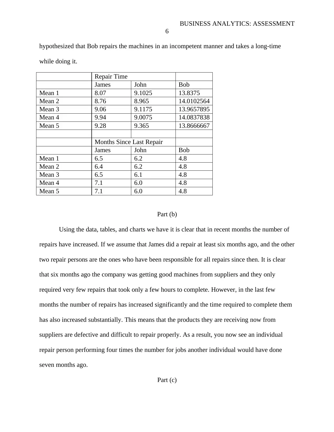
Given that the data is randomly generated we can only assess statistics like mean through
several computations. From the figures below it is clear that James takes the least time to
perform a repair and it is evident that Bob takes the most time when it comes to performing a
task. The table for months since last repair indicate that James has stayed the longest without
being assigned a task; while, bob is the one who has been getting majority of the repair jobs
recently. As such, I would recommend that James be assigned more tasks compared to Bob to
allow for efficiency and diminished downtime will the machine is being fixed. It can also be
5
be moved to another department of be let go, because his productivity level is a quarter of the
other two employees. As such, he should be doing more jobs to ensure that they each perform an
equal 30 repairs.
Mechanical
Jobs
Electrical
Jobs
Total
Jobs
James 4 6 10
John 23 17 40
Bob 17 23 40
Mechanical Jobs Electrical Jobs Total Jobs
0
5
10
15
20
25
30
35
40
45
Repairs
James
John
Bob
Given that the data is randomly generated we can only assess statistics like mean through
several computations. From the figures below it is clear that James takes the least time to
perform a repair and it is evident that Bob takes the most time when it comes to performing a
task. The table for months since last repair indicate that James has stayed the longest without
being assigned a task; while, bob is the one who has been getting majority of the repair jobs
recently. As such, I would recommend that James be assigned more tasks compared to Bob to
allow for efficiency and diminished downtime will the machine is being fixed. It can also be
BUSINESS ANALYTICS: ASSESSMENT
6
hypothesized that Bob repairs the machines in an incompetent manner and takes a long-time
while doing it.
Repair Time
James John Bob
Mean 1 8.07 9.1025 13.8375
Mean 2 8.76 8.965 14.0102564
Mean 3 9.06 9.1175 13.9657895
Mean 4 9.94 9.0075 14.0837838
Mean 5 9.28 9.365 13.8666667
Months Since Last Repair
James John Bob
Mean 1 6.5 6.2 4.8
Mean 2 6.4 6.2 4.8
Mean 3 6.5 6.1 4.8
Mean 4 7.1 6.0 4.8
Mean 5 7.1 6.0 4.8
Part (b)
Using the data, tables, and charts we have it is clear that in recent months the number of
repairs have increased. If we assume that James did a repair at least six months ago, and the other
two repair persons are the ones who have been responsible for all repairs since then. It is clear
that six months ago the company was getting good machines from suppliers and they only
required very few repairs that took only a few hours to complete. However, in the last few
months the number of repairs has increased significantly and the time required to complete them
has also increased substantially. This means that the products they are receiving now from
suppliers are defective and difficult to repair properly. As a result, you now see an individual
repair person performing four times the number for jobs another individual would have done
seven months ago.
Part (c)
⊘ This is a preview!⊘
Do you want full access?
Subscribe today to unlock all pages.

Trusted by 1+ million students worldwide
BUSINESS ANALYTICS: ASSESSMENT
7
The manager can add data regarding the period between one repair and the need for the
same machine. Moreover, the manager can add the identities of the machines that were repaired
to ensure that one can track which products has received the bulk of the repairs. Another dataset
that can also be included is the name of the supplier who sold the business that particular
machine. By so doing, the analysis will reveal which individual has been supplying ineffective
products. In the inclusion of this data will allow for expansive analysis such as logistic regression
and correlation analysis.
Question 7
Part (a)
We can check the identity of the users with missing blood type information and see
whether the individual has donated before or after the specified date. If the person has donate on
another occasion and the blood type is indicate, that value should be replicated in the empty cell
for the same individual since blood type does not change. We can use a COUNTIF function to
assess the frequency of each donor ID, and then use the find box to get the location of the other
donation occasion with the same donor. However, if the person has only donated once a logistic
regression using the available data can be performed to establish a relationship between the other
variables (excluding date) and blood type. We will then use the logistic regression equation to
estimate the blood type for each of the first time donors.
Part (b)
I first extracted all unique donor Ids and copied them to another location on the same
worksheet using the advanced filter feature found under the data tab. I used the SUMIFS
function to sum up the total protein values for each unique donor. After this, I employed the
Paraphrase This Document
Need a fresh take? Get an instant paraphrase of this document with our AI Paraphraser
BUSINESS ANALYTICS: ASSESSMENT
8
COUNTIFS function to compute the frequency of each unique donor in the data. Lastly, I
divided the sum of total protein for each unique donor by their respective frequency.
Part (C).
We first construct a pivot table by selecting the data with Donor ID and Total Protein
Level. We then go to insert tab and select pivot table. We the assign donor Id to row and total
protein level to values. We click on the Sum of Scores drop-down arrow and select value field
setting and change the setting from sum to max. Copy the max values to a column labelled
maximum value and label the adjacent column minimum (go back to the pivot table and change
the value field setting from max to min). Copy the new data to the minimum column. The range
is given by subtracting minimum from maximum for all donors.
Part (d)
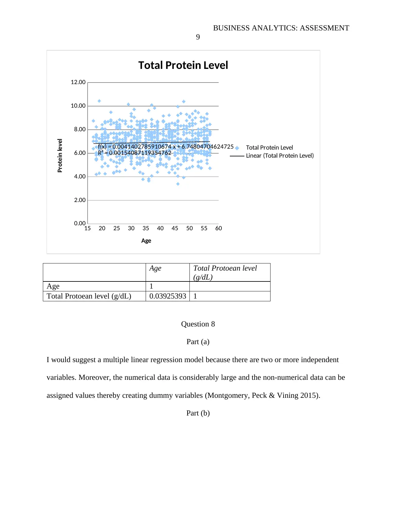
The drawing a X-Y scatter for age against total protein level, suggests that the concentration does
not decline with age. In fact it proposes that it increases by a very small quantity as one gets
older.
Part (e)
BUSINESS ANALYTICS: ASSESSMENT
9
15 20 25 30 35 40 45 50 55 60
0.00
2.00
4.00
6.00
8.00
10.00
12.00
f(x) = 0.0041402785910674 x + 6.74804704624725
R² = 0.00154087119354762
Total Protein Level
Total Protein Level
Linear (Total Protein Level)
Age
Protein level
Age Total Protoean level
(g/dL)
Age 1
Total Protoean level (g/dL) 0.03925393 1
Question 8
Part (a)
I would suggest a multiple linear regression model because there are two or more independent
variables. Moreover, the numerical data is considerably large and the non-numerical data can be
assigned values thereby creating dummy variables (Montgomery, Peck & Vining 2015).
Part (b)
⊘ This is a preview!⊘
Do you want full access?
Subscribe today to unlock all pages.

Trusted by 1+ million students worldwide
BUSINESS ANALYTICS: ASSESSMENT
10
SUMMARY OUTPUT
Regression Statistics
Multiple R 0.90942776
R Square 0.82705885
Adjusted R Square 0.80111768
Standard Error 5.92061899
Observations 24
ANOVA
df SS MS F Significance F
Regression 3 3352.75875 1117.58625 31.8820928 8.1291E-08
Residual 20 701.074585 35.0537293
Total 23 4053.83333
Coefficients Standard Error t Stat P-value Lower 95% Upper 95% Lower 95.0% Upper 95.0%
Intercept -30.3962429 10.9168795 -2.78433438 0.01144652 -53.1684544 -7.62403133 -53.1684544 -7.62403133
Age 0.79998522 0.09233234 8.66419308 3.3274E-08 0.60738334 0.99258711 0.60738334 0.99258711
Weight (Kg) 0.39020608 0.11032607 3.53684371 0.00207062 0.16006992 0.62034224 0.16006992 0.62034224
Gender 5.10871994 2.81094531 1.8174384 0.08416445 -0.75480921 10.9722491 -0.75480921 10.9722491
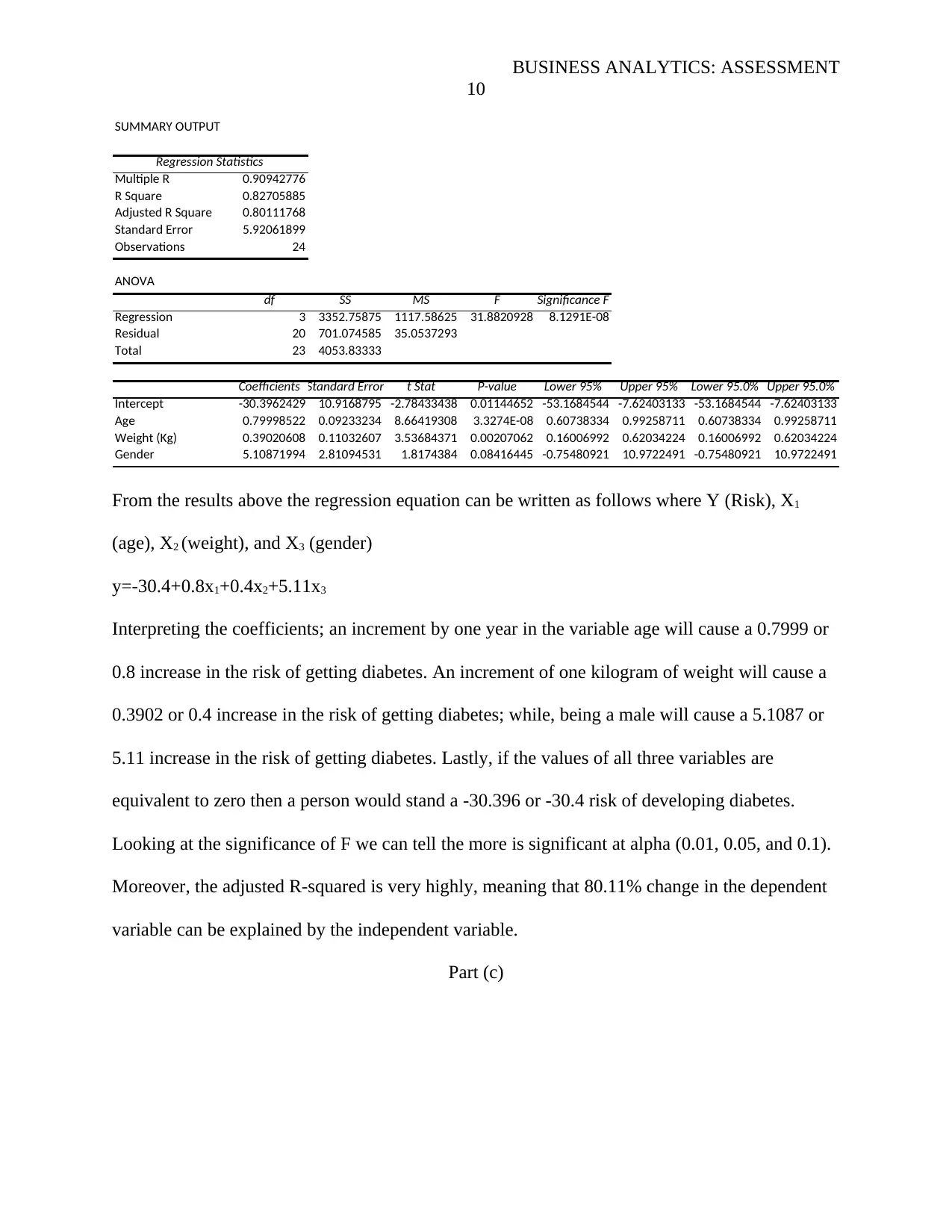
From the results above the regression equation can be written as follows where Y (Risk), X1
(age), X2 (weight), and X3 (gender)
y=-30.4+0.8x1+0.4x2+5.11x3
Interpreting the coefficients; an increment by one year in the variable age will cause a 0.7999 or
0.8 increase in the risk of getting diabetes. An increment of one kilogram of weight will cause a
0.3902 or 0.4 increase in the risk of getting diabetes; while, being a male will cause a 5.1087 or
5.11 increase in the risk of getting diabetes. Lastly, if the values of all three variables are
equivalent to zero then a person would stand a -30.396 or -30.4 risk of developing diabetes.
Looking at the significance of F we can tell the more is significant at alpha (0.01, 0.05, and 0.1).
Moreover, the adjusted R-squared is very highly, meaning that 80.11% change in the dependent
variable can be explained by the independent variable.
Part (c)
Paraphrase This Document
Need a fresh take? Get an instant paraphrase of this document with our AI Paraphraser
BUSINESS ANALYTICS: ASSESSMENT
11
SUMMARY OUTPUT
Regression Statistics
Multiple R 0.91010792
R Square 0.82829642
Adjusted R Square 0.7921483
Standard Error 6.05265362
Observations 24
ANOVA
df SS MS F Significance F
Regression 4 3357.77563 839.443908 22.9139541 4.7673E-07
Residual 19 696.057702 36.6346159
Total 23 4053.83333
Coefficients Standard Error t Stat P-value Lower 95% Upper 95% Lower 95.0% Upper 95.0%
Intercept -29.643719 11.3440861 -2.61314298 0.01709854 -53.387164 -5.90027393 -53.387164 -5.90027393
Age 0.79225611 0.09667457 8.19508253 1.1696E-07 0.5899139 0.99459831 0.5899139 0.99459831
Weight (Kg) 0.38130408 0.11532325 3.30639375 0.0037115 0.13992974 0.62267842 0.13992974 0.62267842
Gender 4.64048051 3.13986742 1.47792244 0.15581467 -1.93133751 11.2122985 -1.93133751 11.2122985
Lifestyle 0.58581131 1.58302063 0.37005918 0.7154313 -2.72748893 3.89911156 -2.72748893 3.89911156
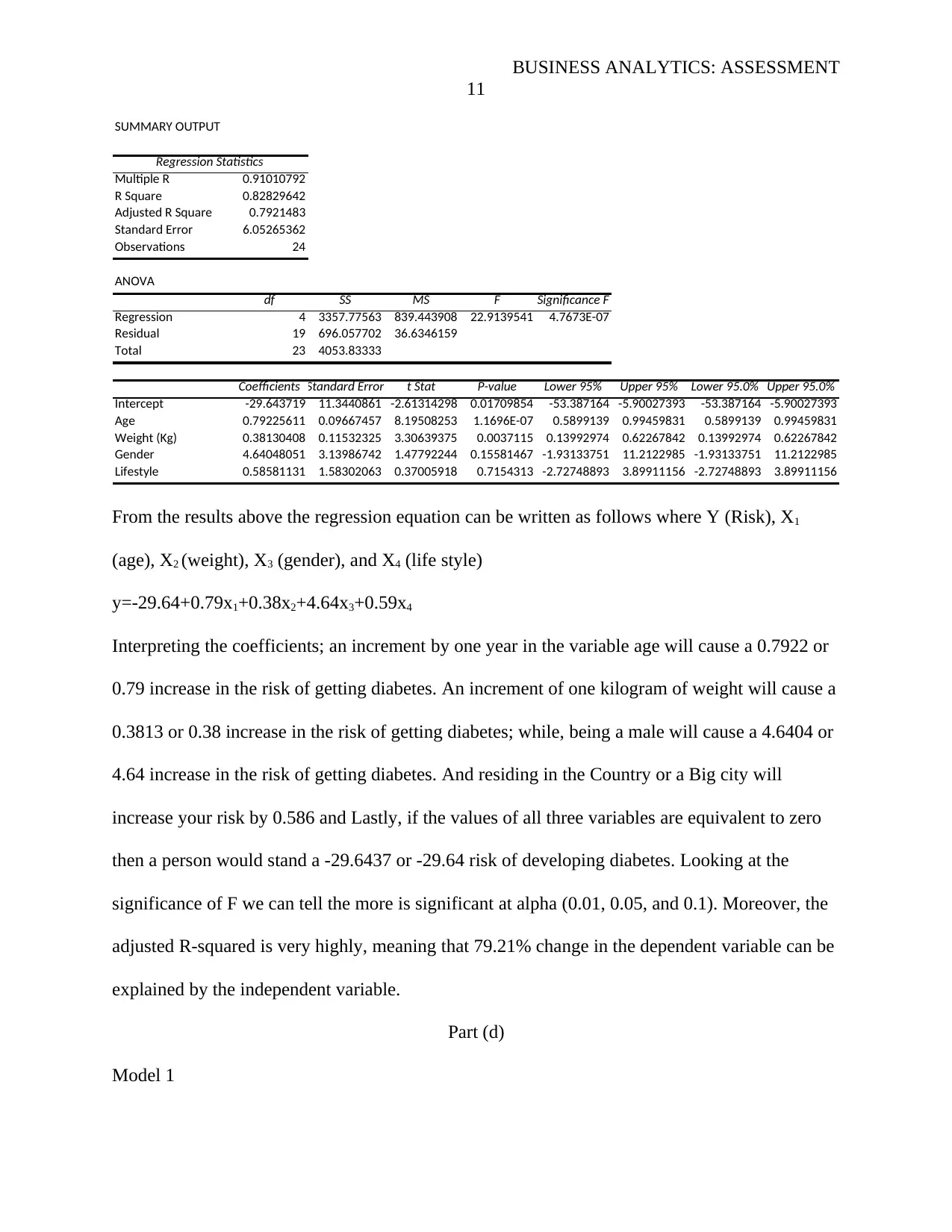
From the results above the regression equation can be written as follows where Y (Risk), X1
(age), X2 (weight), X3 (gender), and X4 (life style)
y=-29.64+0.79x1+0.38x2+4.64x3+0.59x4
Interpreting the coefficients; an increment by one year in the variable age will cause a 0.7922 or
0.79 increase in the risk of getting diabetes. An increment of one kilogram of weight will cause a
0.3813 or 0.38 increase in the risk of getting diabetes; while, being a male will cause a 4.6404 or
4.64 increase in the risk of getting diabetes. And residing in the Country or a Big city will
increase your risk by 0.586 and Lastly, if the values of all three variables are equivalent to zero
then a person would stand a -29.6437 or -29.64 risk of developing diabetes. Looking at the
significance of F we can tell the more is significant at alpha (0.01, 0.05, and 0.1). Moreover, the
adjusted R-squared is very highly, meaning that 79.21% change in the dependent variable can be
explained by the independent variable.
Part (d)
Model 1
BUSINESS ANALYTICS: ASSESSMENT
12
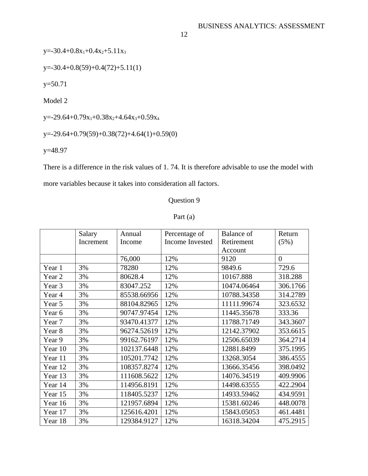
y=-30.4+0.8x1+0.4x2+5.11x3
y=-30.4+0.8(59)+0.4(72)+5.11(1)
y=50.71
Model 2
y=-29.64+0.79x1+0.38x2+4.64x3+0.59x4
y=-29.64+0.79(59)+0.38(72)+4.64(1)+0.59(0)
y=48.97
There is a difference in the risk values of 1. 74. It is therefore advisable to use the model with
more variables because it takes into consideration all factors.
Question 9
Part (a)
Salary
Increment
Annual
Income
Percentage of
Income Invested
Balance of
Retirement
Account
Return
(5%)
76,000 12% 9120 0
Year 1 3% 78280 12% 9849.6 729.6
Year 2 3% 80628.4 12% 10167.888 318.288
Year 3 3% 83047.252 12% 10474.06464 306.1766
Year 4 3% 85538.66956 12% 10788.34358 314.2789
Year 5 3% 88104.82965 12% 11111.99674 323.6532
Year 6 3% 90747.97454 12% 11445.35678 333.36
Year 7 3% 93470.41377 12% 11788.71749 343.3607
Year 8 3% 96274.52619 12% 12142.37902 353.6615
Year 9 3% 99162.76197 12% 12506.65039 364.2714
Year 10 3% 102137.6448 12% 12881.8499 375.1995
Year 11 3% 105201.7742 12% 13268.3054 386.4555
Year 12 3% 108357.8274 12% 13666.35456 398.0492
Year 13 3% 111608.5622 12% 14076.34519 409.9906
Year 14 3% 114956.8191 12% 14498.63555 422.2904
Year 15 3% 118405.5237 12% 14933.59462 434.9591
Year 16 3% 121957.6894 12% 15381.60246 448.0078
Year 17 3% 125616.4201 12% 15843.05053 461.4481
Year 18 3% 129384.9127 12% 16318.34204 475.2915
⊘ This is a preview!⊘
Do you want full access?
Subscribe today to unlock all pages.

Trusted by 1+ million students worldwide
1 out of 17
Related Documents
Your All-in-One AI-Powered Toolkit for Academic Success.
+13062052269
info@desklib.com
Available 24*7 on WhatsApp / Email
![[object Object]](/_next/static/media/star-bottom.7253800d.svg)
Unlock your academic potential
Copyright © 2020–2026 A2Z Services. All Rights Reserved. Developed and managed by ZUCOL.


