Business Analytics - Discussion and Quantitative Questions

This article covers discussion questions on imbalance data, logistic regression, practical examples of logistics regression, and developing a logistics model using categorical variables. It also covers quantitative questions on developing a K Nearest Neighbour Model, predictive analysis, dealing with missing values, calculating averages and range, and visualization tools.

Business Analytics
Institution Name:
Student Name:
Contents
Contents................................................................................................................................................2

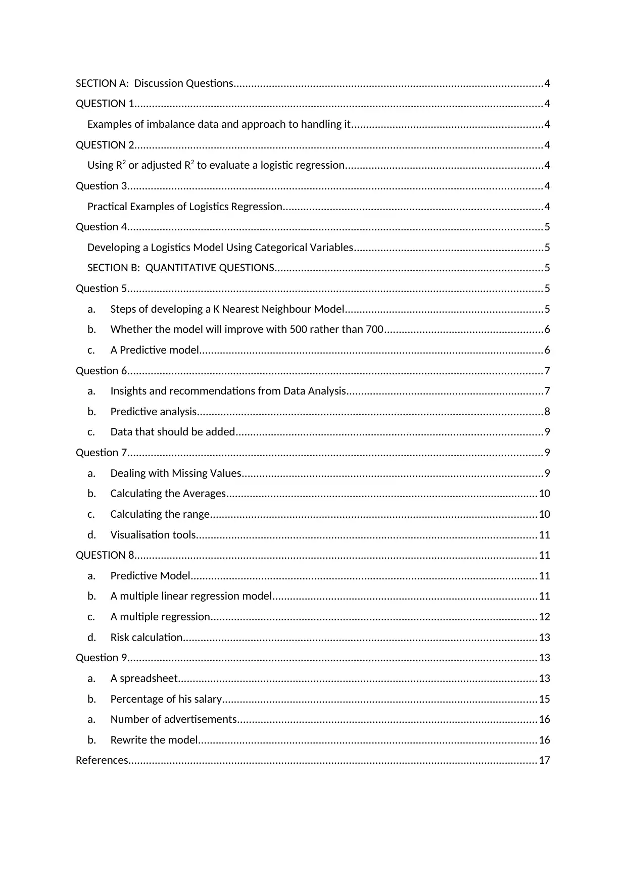
SECTION A: Discussion Questions.........................................................................................................4
QUESTION 1...........................................................................................................................................4
Examples of imbalance data and approach to handling it.................................................................4
QUESTION 2...........................................................................................................................................4
Using R2 or adjusted R2 to evaluate a logistic regression...................................................................4
Question 3.............................................................................................................................................4
Practical Examples of Logistics Regression........................................................................................4
Question 4.............................................................................................................................................5
Developing a Logistics Model Using Categorical Variables................................................................5
SECTION B: QUANTITATIVE QUESTIONS...........................................................................................5
Question 5.............................................................................................................................................5
a. Steps of developing a K Nearest Neighbour Model...................................................................5
b. Whether the model will improve with 500 rather than 700......................................................6
c. A Predictive model.....................................................................................................................6
Question 6.............................................................................................................................................7
a. Insights and recommendations from Data Analysis...................................................................7
b. Predictive analysis.....................................................................................................................8
c. Data that should be added........................................................................................................9
Question 7.............................................................................................................................................9
a. Dealing with Missing Values......................................................................................................9
b. Calculating the Averages..........................................................................................................10
c. Calculating the range...............................................................................................................10
d. Visualisation tools....................................................................................................................11
QUESTION 8.........................................................................................................................................11
a. Predictive Model......................................................................................................................11
b. A multiple linear regression model..........................................................................................11
c. A multiple regression...............................................................................................................12
d. Risk calculation........................................................................................................................13
Question 9...........................................................................................................................................13
a. A spreadsheet..........................................................................................................................13
b. Percentage of his salary...........................................................................................................15
a. Number of advertisements......................................................................................................16
b. Rewrite the model...................................................................................................................16
References...........................................................................................................................................17

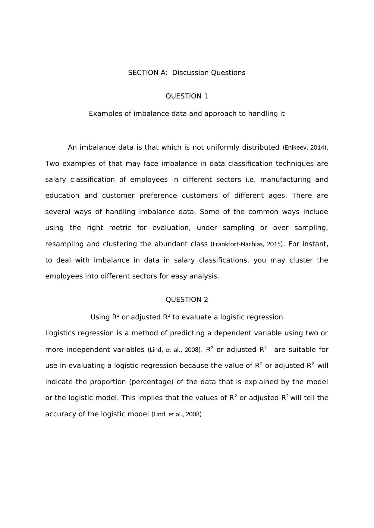
SECTION A: Discussion Questions
QUESTION 1
Examples of imbalance data and approach to handling it
An imbalance data is that which is not uniformly distributed (Enikeev, 2014).
Two examples of that may face imbalance in data classification techniques are
salary classification of employees in different sectors i.e. manufacturing and
education and customer preference customers of different ages. There are
several ways of handling imbalance data. Some of the common ways include
using the right metric for evaluation, under sampling or over sampling,
resampling and clustering the abundant class (Frankfort-Nachias, 2015). For instant,
to deal with imbalance in data in salary classifications, you may cluster the
employees into different sectors for easy analysis.
QUESTION 2
Using R2 or adjusted R2 to evaluate a logistic regression
Logistics regression is a method of predicting a dependent variable using two or
more independent variables (Lind, et al., 2008). R2 or adjusted R2 are suitable for
use in evaluating a logistic regression because the value of R2 or adjusted R2 will
indicate the proportion (percentage) of the data that is explained by the model
or the logistic model. This implies that the values of R2 or adjusted R2 will tell the
accuracy of the logistic model (Lind, et al., 2008)

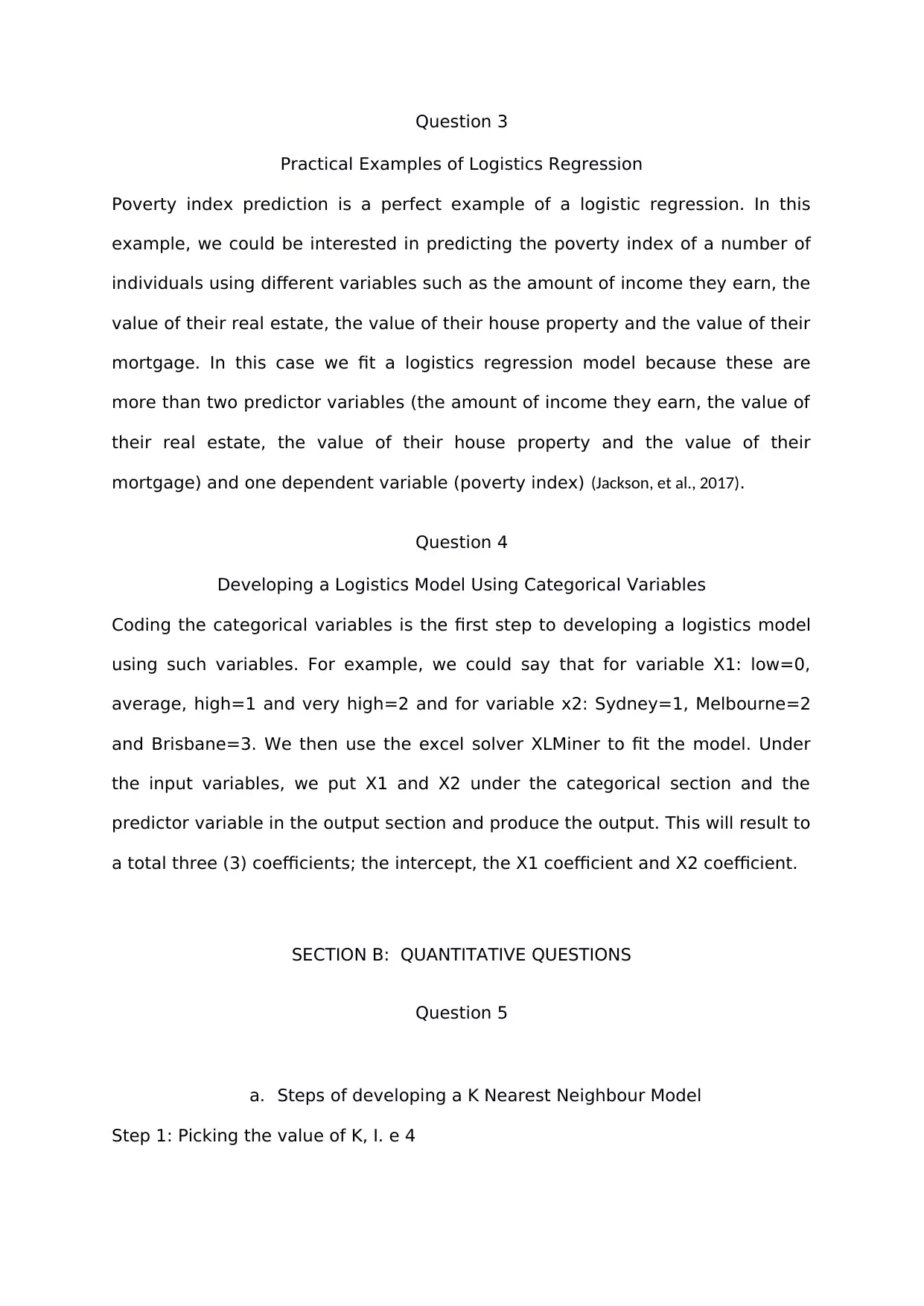
Question 3
Practical Examples of Logistics Regression
Poverty index prediction is a perfect example of a logistic regression. In this
example, we could be interested in predicting the poverty index of a number of
individuals using different variables such as the amount of income they earn, the
value of their real estate, the value of their house property and the value of their
mortgage. In this case we fit a logistics regression model because these are
more than two predictor variables (the amount of income they earn, the value of
their real estate, the value of their house property and the value of their
mortgage) and one dependent variable (poverty index) (Jackson, et al., 2017).
Question 4
Developing a Logistics Model Using Categorical Variables
Coding the categorical variables is the first step to developing a logistics model
using such variables. For example, we could say that for variable X1: low=0,
average, high=1 and very high=2 and for variable x2: Sydney=1, Melbourne=2
and Brisbane=3. We then use the excel solver XLMiner to fit the model. Under
the input variables, we put X1 and X2 under the categorical section and the
predictor variable in the output section and produce the output. This will result to
a total three (3) coefficients; the intercept, the X1 coefficient and X2 coefficient.
SECTION B: QUANTITATIVE QUESTIONS
Question 5
a. Steps of developing a K Nearest Neighbour Model
Step 1: Picking the value of K, I. e 4

Step 2: Searching for values that nearest to the chosen value k
Step 3: calculating the distance between the test data and the training row
Step 4: Arrange the calculated distances in ascending order
Step 5: Sort, get the frequent value of k and get the most frequent value of k.
b. Whether the model will improve with 500 rather than 700
No, the model will not improve. The improvement of the model depends on the
value of k and the number of iterations and not the value being predicted (Enikeev,
2014).
c. A Predictive model
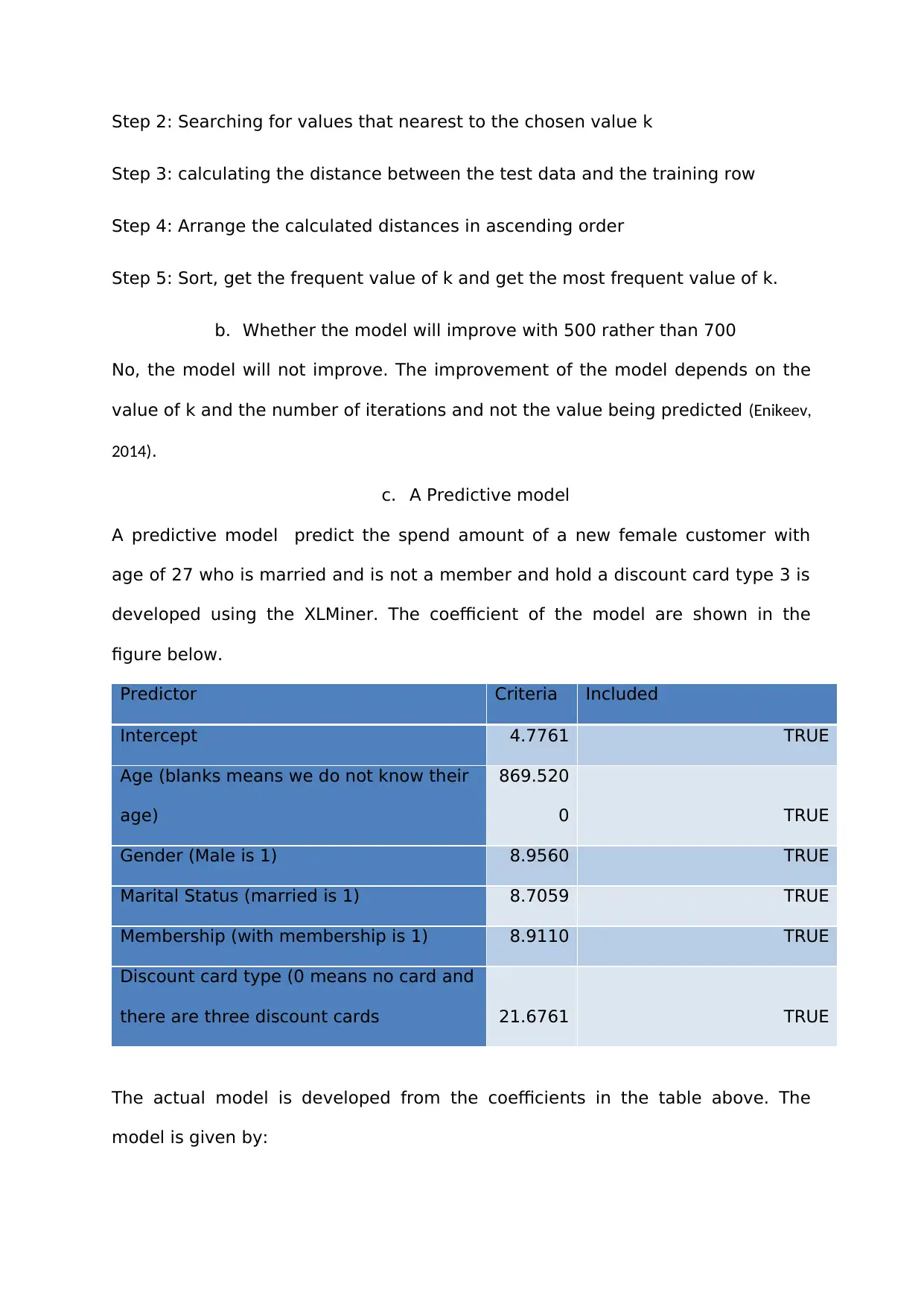
A predictive model predict the spend amount of a new female customer with
age of 27 who is married and is not a member and hold a discount card type 3 is
developed using the XLMiner. The coefficient of the model are shown in the
figure below.
Predictor Criteria Included
Intercept 4.7761 TRUE
Age (blanks means we do not know their
age)
869.520
0 TRUE
Gender (Male is 1) 8.9560 TRUE
Marital Status (married is 1) 8.7059 TRUE
Membership (with membership is 1) 8.9110 TRUE
Discount card type (0 means no card and
there are three discount cards 21.6761 TRUE
The actual model is developed from the coefficients in the table above. The
model is given by:

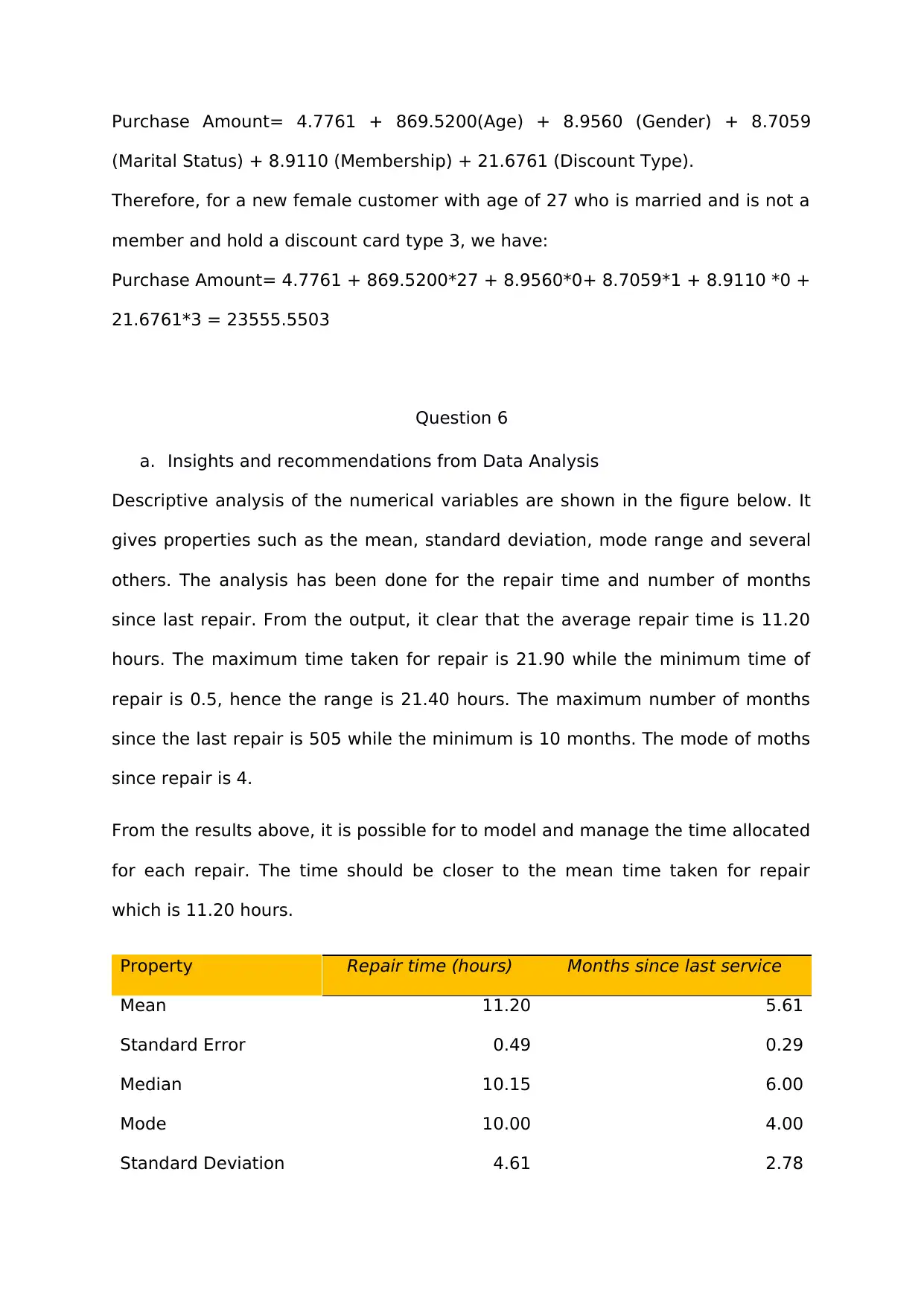
Purchase Amount= 4.7761 + 869.5200(Age) + 8.9560 (Gender) + 8.7059
(Marital Status) + 8.9110 (Membership) + 21.6761 (Discount Type).
Therefore, for a new female customer with age of 27 who is married and is not a
member and hold a discount card type 3, we have:
Purchase Amount= 4.7761 + 869.5200*27 + 8.9560*0+ 8.7059*1 + 8.9110 *0 +
21.6761*3 = 23555.5503
Question 6
a. Insights and recommendations from Data Analysis
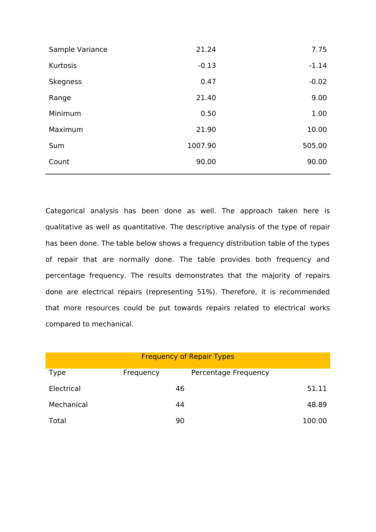
Descriptive analysis of the numerical variables are shown in the figure below. It
gives properties such as the mean, standard deviation, mode range and several
others. The analysis has been done for the repair time and number of months
since last repair. From the output, it clear that the average repair time is 11.20
hours. The maximum time taken for repair is 21.90 while the minimum time of
repair is 0.5, hence the range is 21.40 hours. The maximum number of months
since the last repair is 505 while the minimum is 10 months. The mode of moths
since repair is 4.
From the results above, it is possible for to model and manage the time allocated
for each repair. The time should be closer to the mean time taken for repair
which is 11.20 hours.
Property Repair time (hours) Months since last service
Mean 11.20 5.61
Standard Error 0.49 0.29
Median 10.15 6.00
Mode 10.00 4.00
Standard Deviation 4.61 2.78

Sample Variance 21.24 7.75
Kurtosis -0.13 -1.14
Skegness 0.47 -0.02
Range 21.40 9.00
Minimum 0.50 1.00
Maximum 21.90 10.00
Sum 1007.90 505.00
Count 90.00 90.00
Categorical analysis has been done as well. The approach taken here is
qualitative as well as quantitative. The descriptive analysis of the type of repair
has been done. The table below shows a frequency distribution table of the types
of repair that are normally done. The table provides both frequency and
percentage frequency. The results demonstrates that the majority of repairs
done are electrical repairs (representing 51%). Therefore, it is recommended
that more resources could be put towards repairs related to electrical works
compared to mechanical.
Frequency of Repair Types
Type Frequency Percentage Frequency
Electrical 46 51.11
Mechanical 44 48.89
Total 90 100.00

b. Predictive analysis
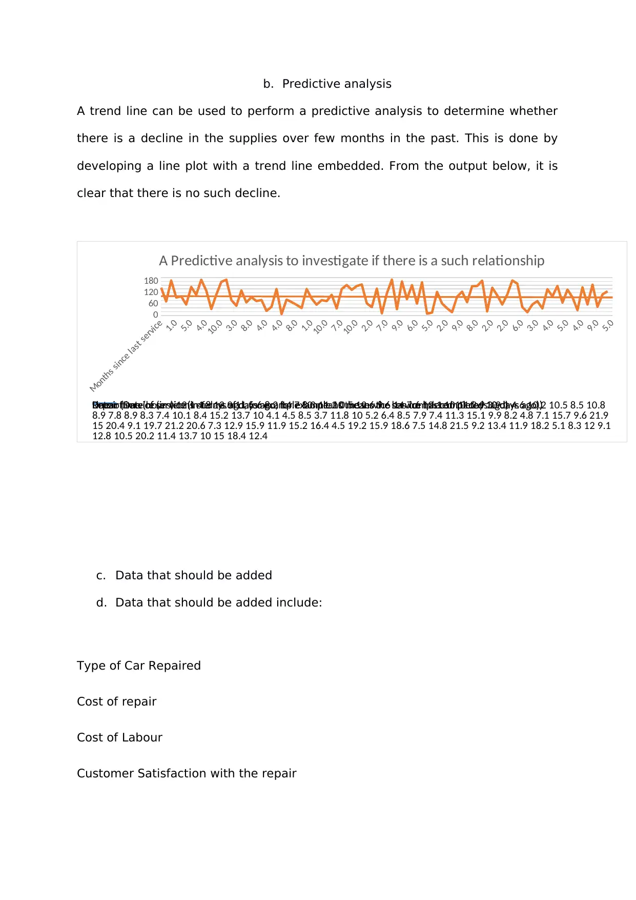
A trend line can be used to perform a predictive analysis to determine whether
there is a decline in the supplies over few months in the past. This is done by
developing a line plot with a trend line embedded. From the output below, it is
clear that there is no such decline.
Months since last service
1.0
5.0
4.0
10.0
3.0
8.0
4.0
4.0
8.0
1.0
10.0
7.0
10.0
2.0
7.0
9.0
6.0
5.0
2.0
9.0
8.0
2.0
2.0
6.0
3.0
4.0
5.0
4.0
9.0
5.0
0
60
120
180
A Predictive analysis to investigate if there is a such relationship
Date of service (in terms of days ago, for example 10 means the service has completed 10 days ago)Linear (Date of service (in terms of days ago, for example 10 means the service has completed 10 days ago))Linear (Date of service (in terms of days ago, for example 10 means the service has completed 10 days ago))Repair time (hours) 12.1 4.8 12.9 11.6 6 8.2 14.7 8.3 11.2 0.5 12.6 9.6 14 7.6 10.1 10 11.2 9.3 9.1 4.6 10.2 10.5 8.5 10.8
8.9 7.8 8.9 8.3 7.4 10.1 8.4 15.2 13.7 10 4.1 4.5 8.5 3.7 11.8 10 5.2 6.4 8.5 7.9 7.4 11.3 15.1 9.9 8.2 4.8 7.1 15.7 9.6 21.9
15 20.4 9.1 19.7 21.2 20.6 7.3 12.9 15.9 11.9 15.2 16.4 4.5 19.2 15.9 18.6 7.5 14.8 21.5 9.2 13.4 11.9 18.2 5.1 8.3 12 9.1
12.8 10.5 20.2 11.4 13.7 10 15 18.4 12.4
c. Data that should be added
d. Data that should be added include:
Type of Car Repaired
Cost of repair
Cost of Labour
Customer Satisfaction with the repair

Question 7
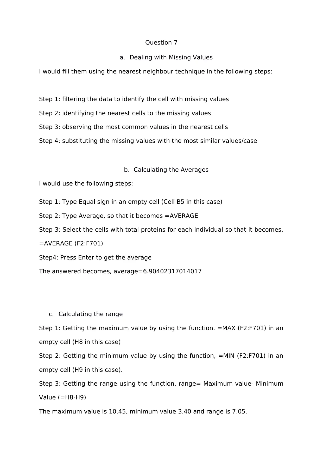
a. Dealing with Missing Values
I would fill them using the nearest neighbour technique in the following steps:
Step 1: filtering the data to identify the cell with missing values
Step 2: identifying the nearest cells to the missing values
Step 3: observing the most common values in the nearest cells
Step 4: substituting the missing values with the most similar values/case
b. Calculating the Averages
I would use the following steps:
Step 1: Type Equal sign in an empty cell (Cell B5 in this case)
Step 2: Type Average, so that it becomes =AVERAGE
Step 3: Select the cells with total proteins for each individual so that it becomes,
=AVERAGE (F2:F701)
Step4: Press Enter to get the average
The answered becomes, average=6.90402317014017
c. Calculating the range
Step 1: Getting the maximum value by using the function, =MAX (F2:F701) in an
empty cell (H8 in this case)
Step 2: Getting the minimum value by using the function, =MIN (F2:F701) in an
empty cell (H9 in this case).
Step 3: Getting the range using the function, range= Maximum value- Minimum
Value (=H8-H9)
The maximum value is 10.45, minimum value 3.40 and range is 7.05.

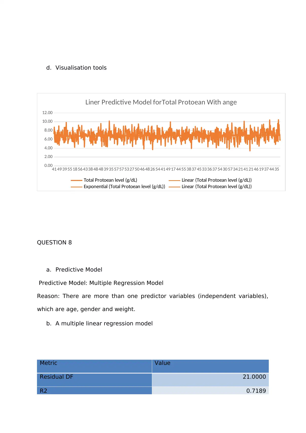
d. Visualisation tools
41 49 39 55 18 56 43 38 48 48 39 35 57 57 53 27 50 46 48 26 54 41 49 17 44 55 38 37 45 33 36 37 54 30 57 34 21 41 21 46 19 37 44 35
0.00
2.00
4.00
6.00
8.00
10.00
12.00
Liner Predictive Model forTotal Protoean With ange
Total Protoean level (g/dL) Linear (Total Protoean level (g/dL))
Exponential (Total Protoean level (g/dL)) Linear (Total Protoean level (g/dL))
QUESTION 8
a. Predictive Model
Predictive Model: Multiple Regression Model
Reason: There are more than one predictor variables (independent variables),
which are age, gender and weight.
b. A multiple linear regression model
Metric Value
Residual DF 21.0000
R2 0.7189

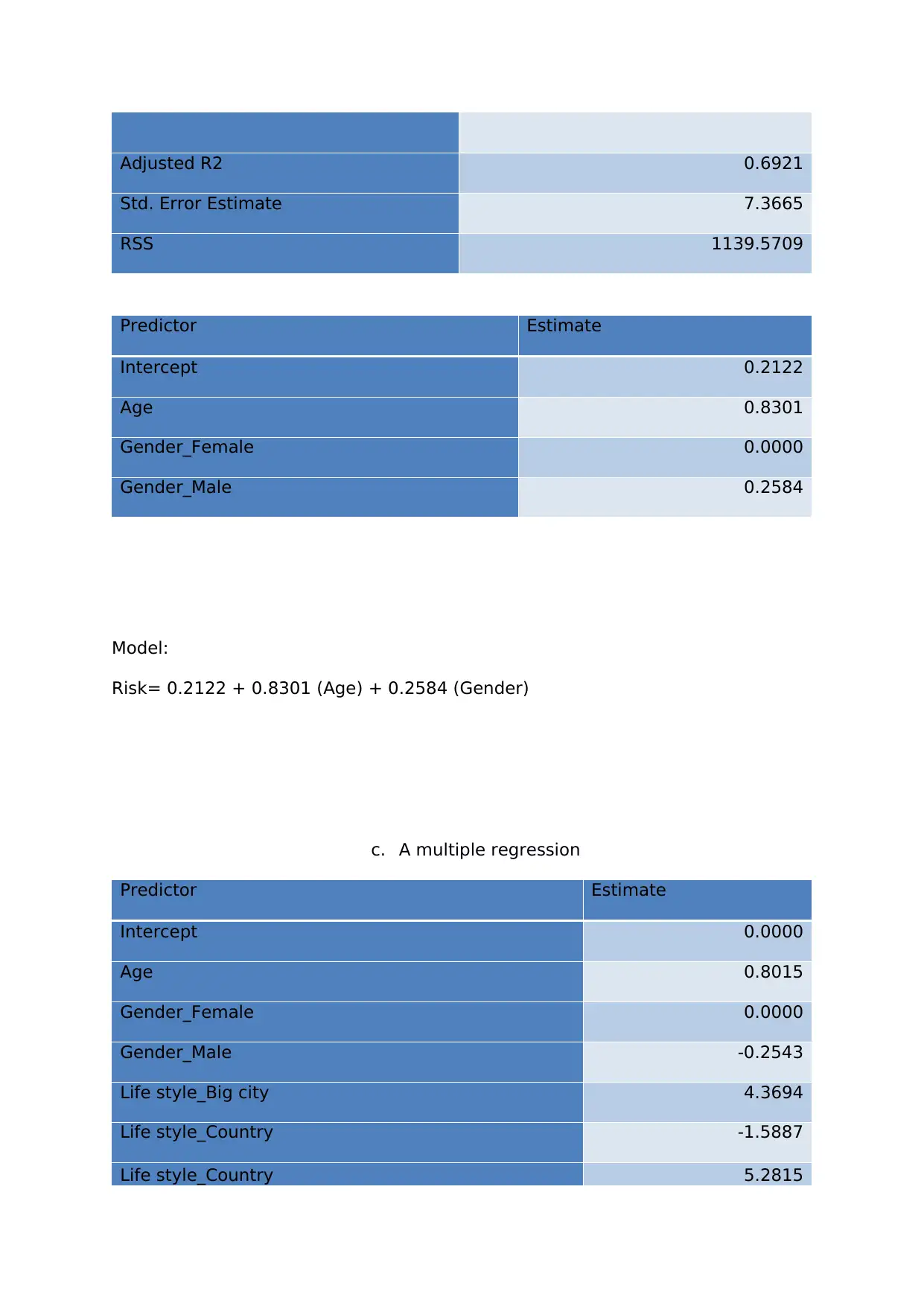
Adjusted R2 0.6921
Std. Error Estimate 7.3665
RSS 1139.5709
Predictor Estimate
Intercept 0.2122
Age 0.8301
Gender_Female 0.0000
Gender_Male 0.2584
Model:
Risk= 0.2122 + 0.8301 (Age) + 0.2584 (Gender)
c. A multiple regression
Predictor Estimate
Intercept 0.0000
Age 0.8015
Gender_Female 0.0000
Gender_Male -0.2543
Life style_Big city 4.3694
Life style_Country -1.5887
Life style_Country 5.2815

Life style_Small town 1.8014
Metric Value
Residual DF 18.0000
R2 0.7506
Adjusted R2 0.6814
Std. Error Estimate 7.4940
RSS 1010.8738
d. Risk calculation
Risk= 0.2122 + 0.8301 (Age) + 0.2584 (Gender)
Question 9
a. A spreadsheet
Time (t) Amount Invested (12%0f After Tax Salary) Retirement Amount
0 9120.00 9120.00
1 9576.00 10054.80
2 10054.80 11085.42
3 10557.54 12221.67
4 11085.42 13474.39

5 11639.69 14855.52
6 12221.67 16378.21
7 12832.76 18056.98
8 13474.39 19907.82
9 14148.11 21948.37
10 14855.52 24198.08
11 15598.29 26678.38
12 16378.21 29412.91
13 17197.12 32427.73
14 18056.98 35751.58
15 18959.82 39416.11
16 19907.82 43456.27
17 20903.21 47910.53
18 21948.37 52821.36
19 23045.79 58235.55
20 24198.08 64204.70
21 25407.98 70785.68
22 26678.38 78041.21
23 28012.30 86040.43
24 29412.91 94859.58
25 30883.56 104582.69
26 32427.73 115302.41
27 34049.12 127120.91
28 35751.58 140150.80
29 37539.16 154516.26
30 39416.11 170354.18

b. Percentage of his salary
Percentage amount= {(1,500,000)/ {(76000*(1.05) ^30)}}
= 4.57%
Question 10
Limitations Website A Website B Website C
Estimated number of
viewers per each
advertisement
130,000 35,000 80,000
Cost per advertisement
for the first 5
advertisements
$2,500
$500 $800
Cost per advertisement
for more than 5
advertisements
$2,200
Maximum acceptable
number of
15 20 35

advertisements
a. Number of advertisements
Maximum acceptable number of advertisements
A 2
B 3
C 4
b. Rewrite the model
Maximum acceptable number of advertisements
A 1
B 4
C 2
References
Enikeev, K. R., 2014. Appliance of Smart Methods for Data Analysis in Online Advertising. 18(09), p.
3.
Frankfort-Nachias, C. &. L.-G. A., 2015. Social Statistics for a diverse society. Thousand Oaks, CA: Sage
Publications.

Jackson, S. et al., 2017. Methods. [Online]
Available at: http://writing.colostate.edu/research/stats/
Lind, D. A., Marchel, W. G. & Wathen, S. A., 2008. Statistical Techniques in Business &. Boston.:
McGraw-Hill Irwin.