Business Data Analysis Question and Answer 2022

Running head: BUSINESS DATA ANALYSIS
BUSINESS DATA ANALYSIS
Name of the Student
Name of the University
Author Note

1BUSINESS DATA ANALYSIS
Question 1:
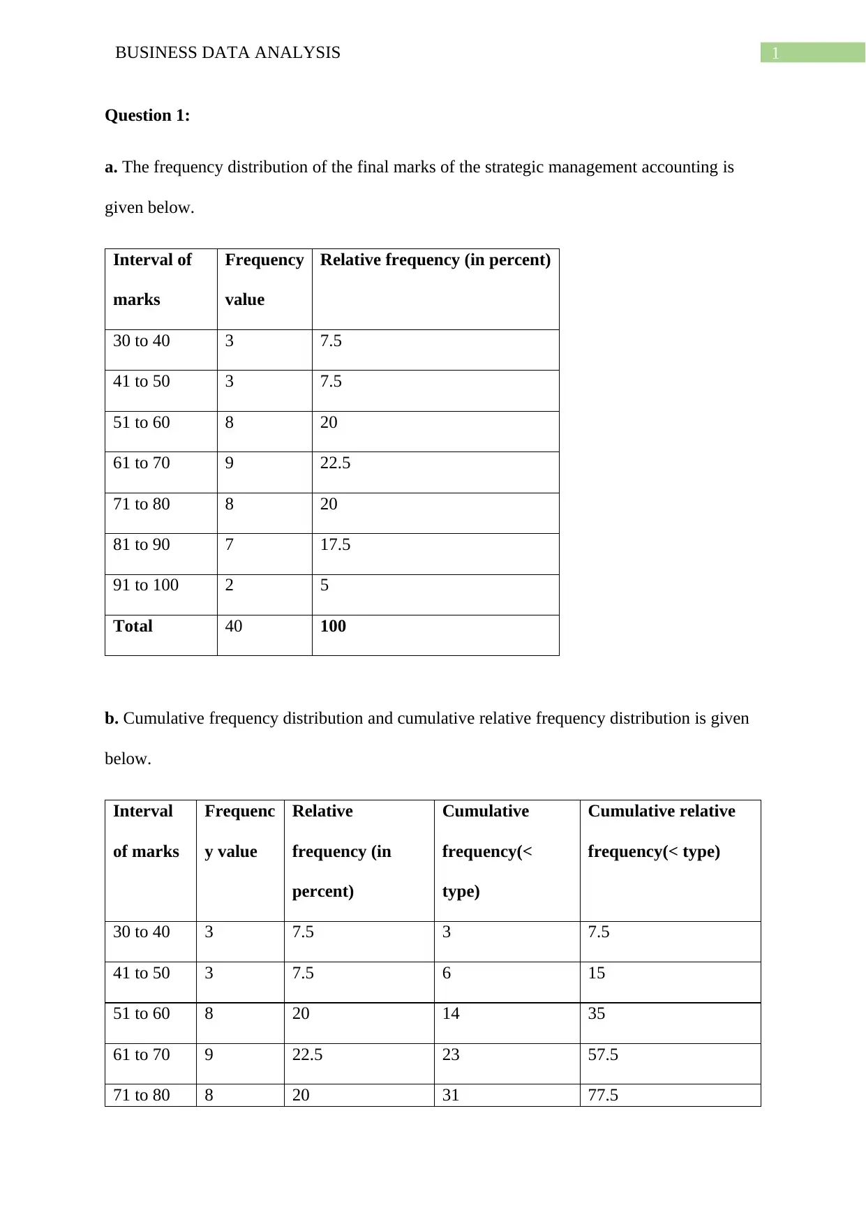
a. The frequency distribution of the final marks of the strategic management accounting is
given below.
Interval of
marks
Frequency
value
Relative frequency (in percent)
30 to 40 3 7.5
41 to 50 3 7.5
51 to 60 8 20
61 to 70 9 22.5
71 to 80 8 20
81 to 90 7 17.5
91 to 100 2 5
Total 40 100
b. Cumulative frequency distribution and cumulative relative frequency distribution is given
below.
Interval
of marks
Frequenc
y value
Relative
frequency (in
percent)
Cumulative
frequency(<
type)
Cumulative relative
frequency(< type)
30 to 40 3 7.5 3 7.5
41 to 50 3 7.5 6 15
51 to 60 8 20 14 35
61 to 70 9 22.5 23 57.5
71 to 80 8 20 31 77.5

2BUSINESS DATA ANALYSIS
81 to 90 7 17.5 38 95
91 to 100 2 5 40 100
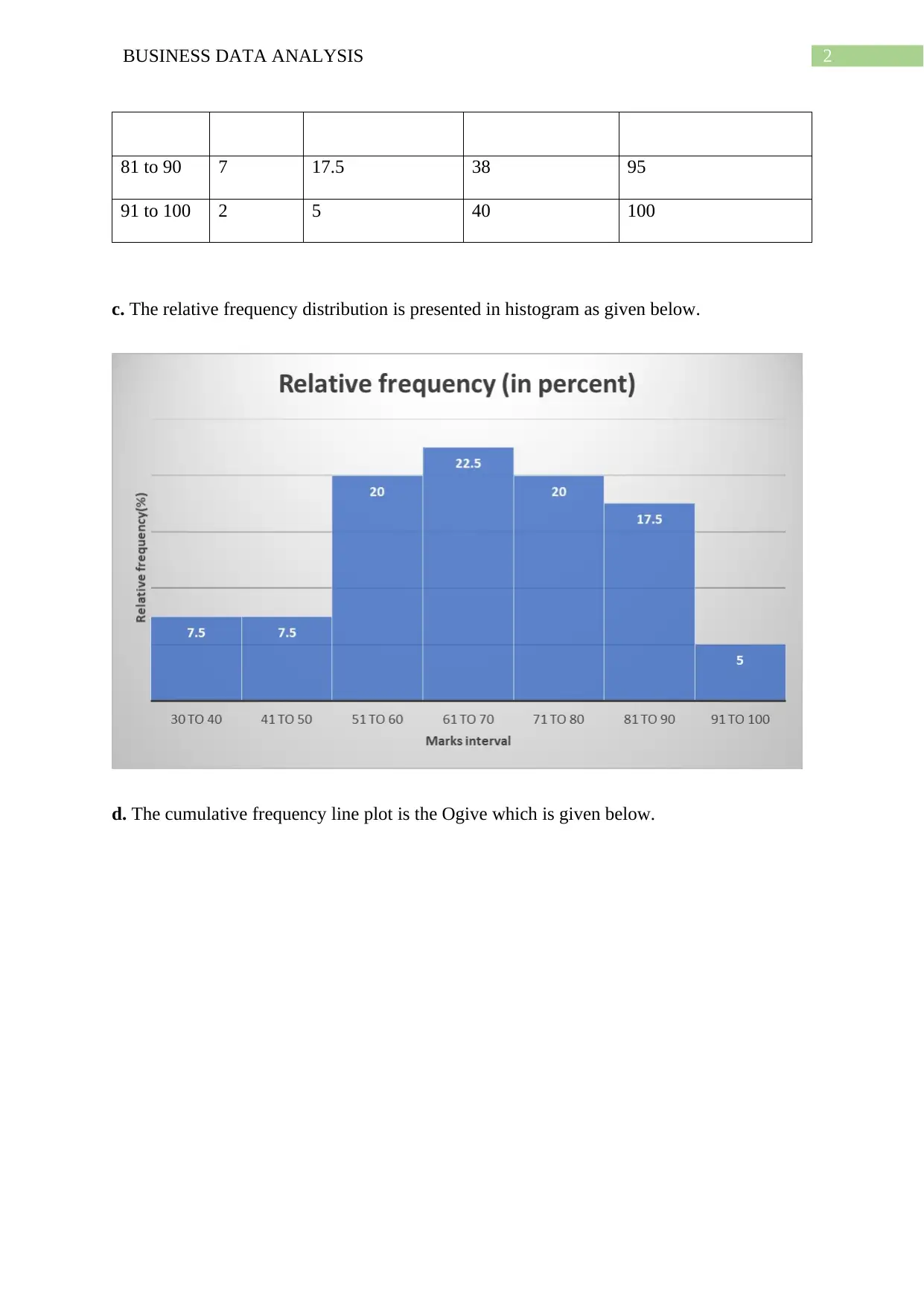
c. The relative frequency distribution is presented in histogram as given below.
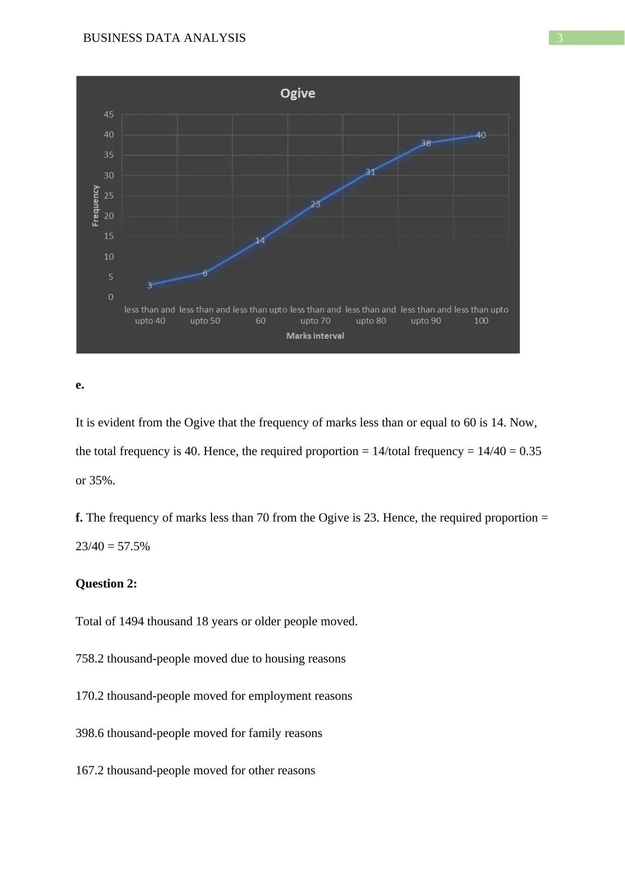
d. The cumulative frequency line plot is the Ogive which is given below.

3BUSINESS DATA ANALYSIS
e.
It is evident from the Ogive that the frequency of marks less than or equal to 60 is 14. Now,
the total frequency is 40. Hence, the required proportion = 14/total frequency = 14/40 = 0.35
or 35%.
f. The frequency of marks less than 70 from the Ogive is 23. Hence, the required proportion =
23/40 = 57.5%
Question 2:
Total of 1494 thousand 18 years or older people moved.
758.2 thousand-people moved due to housing reasons
170.2 thousand-people moved for employment reasons
398.6 thousand-people moved for family reasons
167.2 thousand-people moved for other reasons

4BUSINESS DATA ANALYSIS
Summarized in the following table.
Reason for
leaving
Number of people(in
thousands)
housing 758.2
employment 170.2
family 398.6
other 167.2
a.
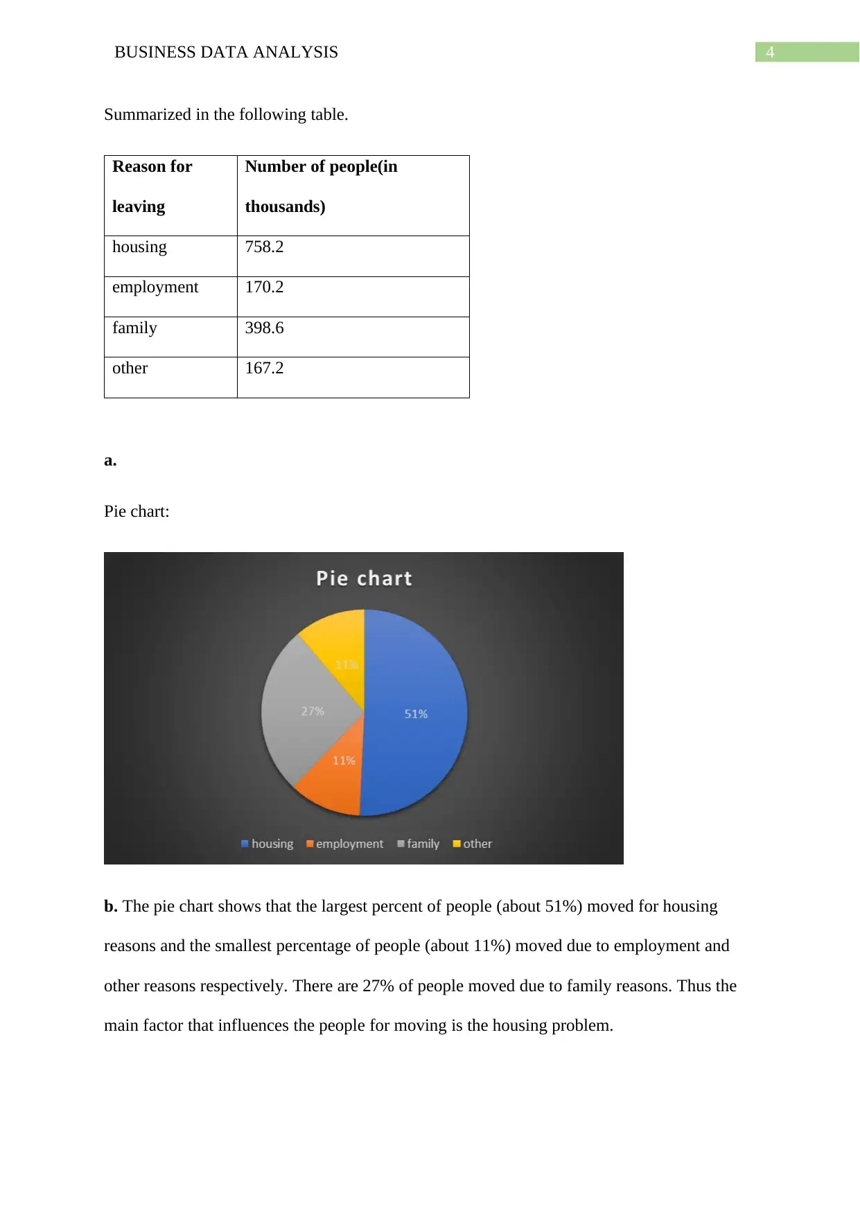
Pie chart:
b. The pie chart shows that the largest percent of people (about 51%) moved for housing
reasons and the smallest percentage of people (about 11%) moved due to employment and
other reasons respectively. There are 27% of people moved due to family reasons. Thus the
main factor that influences the people for moving is the housing problem.

5BUSINESS DATA ANALYSIS
Question 3:
1.
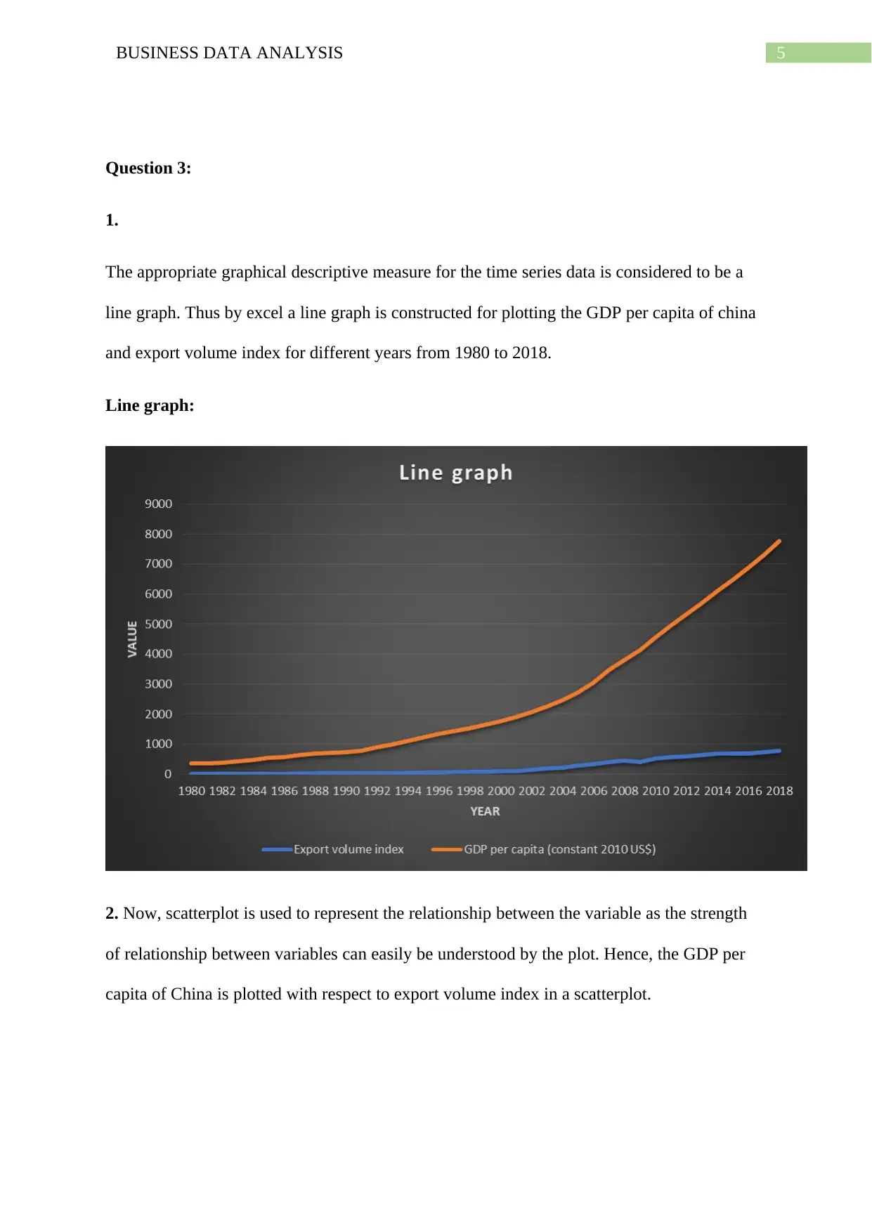
The appropriate graphical descriptive measure for the time series data is considered to be a
line graph. Thus by excel a line graph is constructed for plotting the GDP per capita of china
and export volume index for different years from 1980 to 2018.
Line graph:
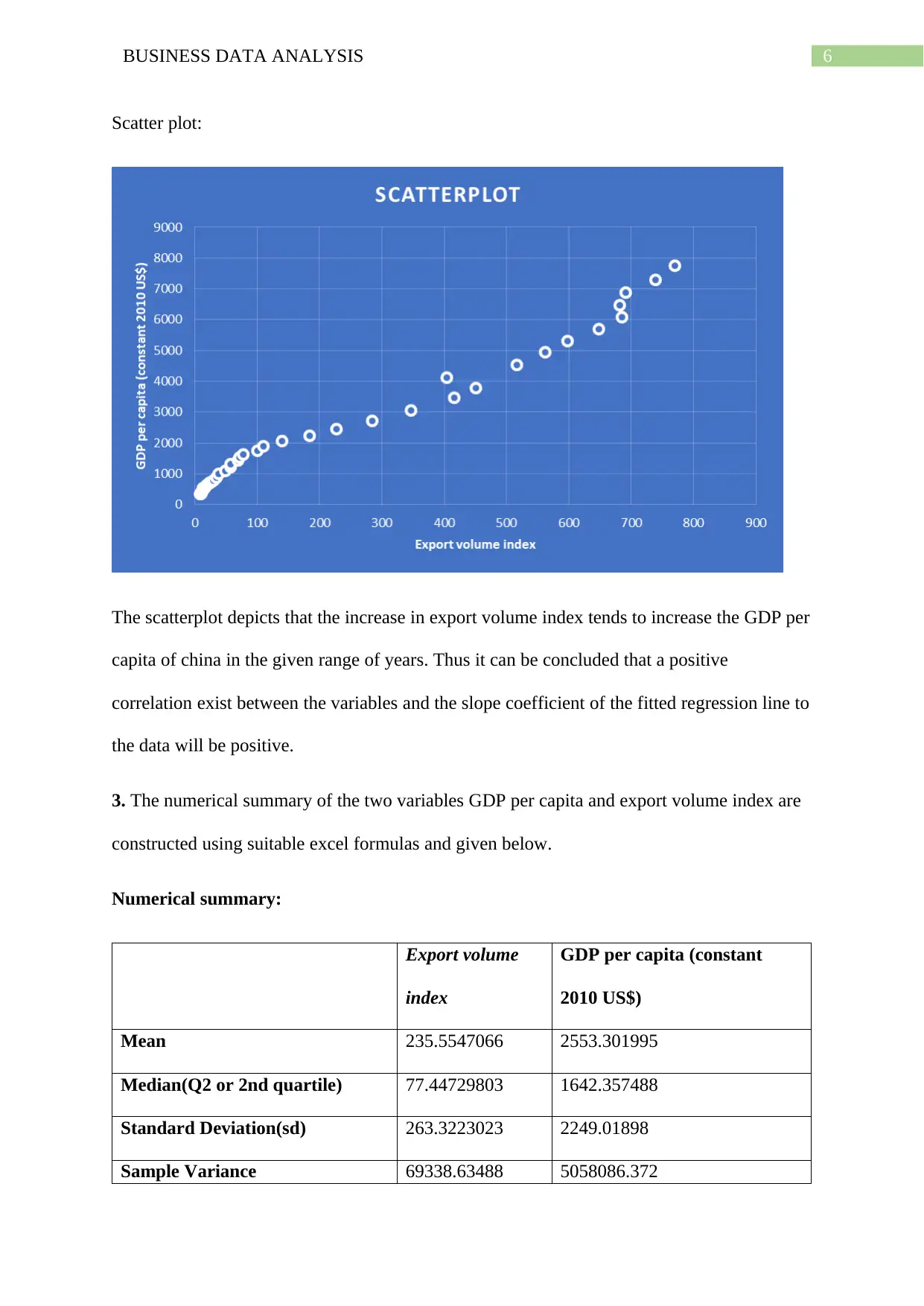
2. Now, scatterplot is used to represent the relationship between the variable as the strength
of relationship between variables can easily be understood by the plot. Hence, the GDP per
capita of China is plotted with respect to export volume index in a scatterplot.

6BUSINESS DATA ANALYSIS
Scatter plot:
The scatterplot depicts that the increase in export volume index tends to increase the GDP per
capita of china in the given range of years. Thus it can be concluded that a positive
correlation exist between the variables and the slope coefficient of the fitted regression line to
the data will be positive.
3. The numerical summary of the two variables GDP per capita and export volume index are
constructed using suitable excel formulas and given below.
Numerical summary:
Export volume
index
GDP per capita (constant
2010 US$)
Mean 235.5547066 2553.301995
Median(Q2 or 2nd quartile) 77.44729803 1642.357488
Standard Deviation(sd) 263.3223023 2249.01898
Sample Variance 69338.63488 5058086.372

7BUSINESS DATA ANALYSIS
Range 762.3573052 7407.842031
Minimum 7.190964398 347.1200879
Maximum 769.5482696 7754.962119
Q1(1st quartile) 22.42809652 712.1153633
Q3(3rd quartile) 450.2958821 4132.902312
Coefficient of Variation(CV
=sd/mean )
1.117881727 0.880827644
4.
The CORREL function is used to calculate the correlation coefficient between the two
variables in excel.
Correlation
coefficient(r)
0.990115538
As the value of the correlation coefficient is approximately equal to 1, hence the GDP per
capita and export volume index are strongly positive correlated.
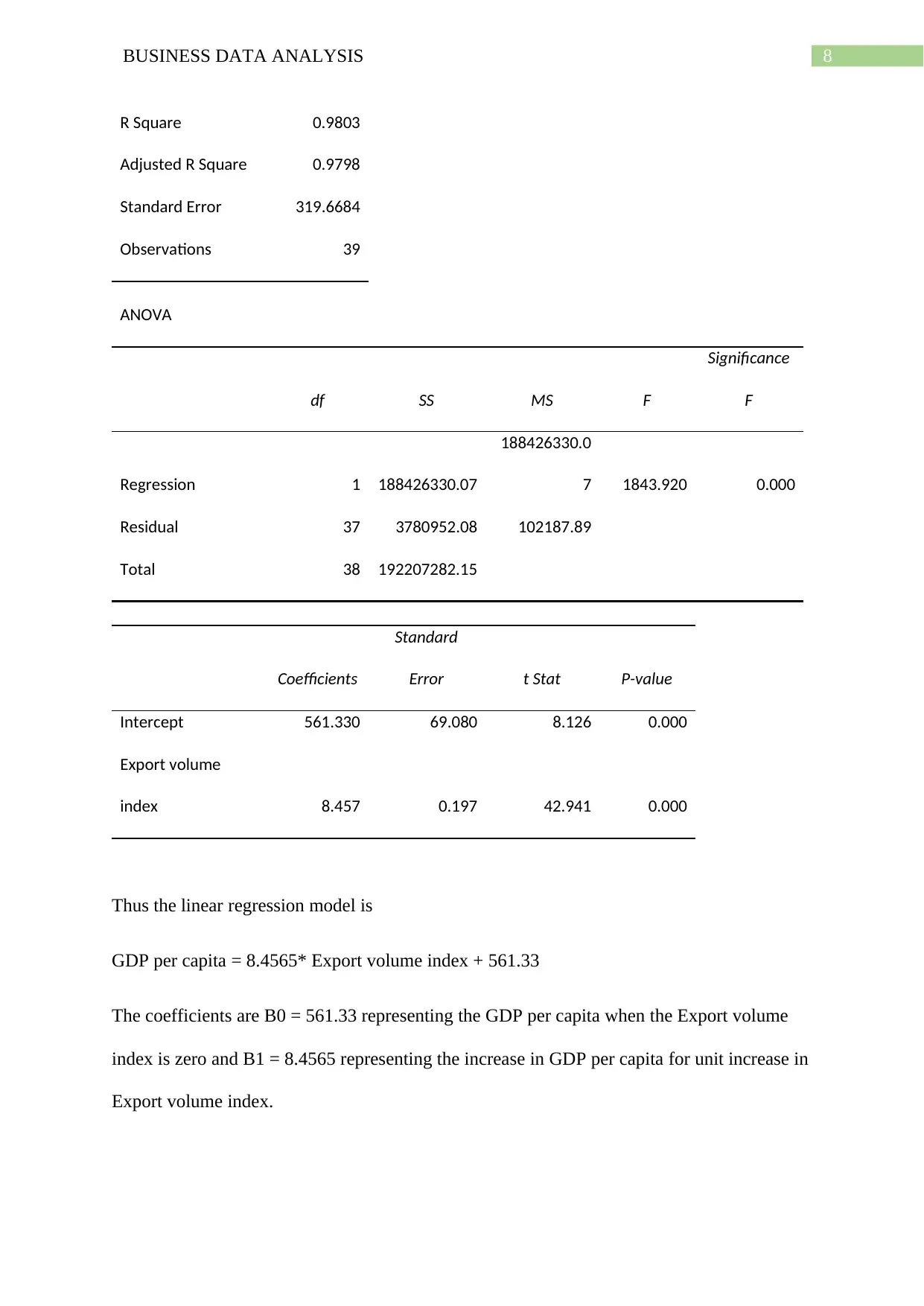
5. The regression analysis is performed by using data analysis toolbar in excel and the result
is shown below.
SUMMARY OUTPUT
Regression Statistics
Multiple R 0.9901

8BUSINESS DATA ANALYSIS
R Square 0.9803
Adjusted R Square 0.9798
Standard Error 319.6684
Observations 39
ANOVA
df SS MS F
Significance
F
Regression 1 188426330.07
188426330.0
7 1843.920 0.000
Residual 37 3780952.08 102187.89
Total 38 192207282.15
Coefficients
Standard
Error t Stat P-value
Intercept 561.330 69.080 8.126 0.000
Export volume
index 8.457 0.197 42.941 0.000
Thus the linear regression model is
GDP per capita = 8.4565* Export volume index + 561.33
The coefficients are B0 = 561.33 representing the GDP per capita when the Export volume
index is zero and B1 = 8.4565 representing the increase in GDP per capita for unit increase in
Export volume index.

9BUSINESS DATA ANALYSIS
The coefficient of export volume index of the equation is 8.4565 which indicates for unit
increase in Export volume index the GDP per capita is increased by 8.4565 (in constant 2010
US$) and the intercept 561.33 indicates that when the export volume index is zero then GDP
per capita is 561.33 (in constant 2010 US$).
6. The value of coefficient of determination R2 = 0.9803 as found from the regression table.
This value indicates that almost 98.03% of variation in GDP per capita of China is explained
by the variation of Export volume index and the rest 1.97% of variation is unexplained by the
regression model. This unexplained variation is either caused by other variables which are not
included in the regression model or is caused by random error or both.
7.
Now, as seen from the regression output table the coefficient of Export volume index is
positive and the p value of this is significant as it is less than given significance level of 0.05.
Hence, it can be stated that GDP per capita is positively and significantly increases with
export volume index.
8. The standard error is given by,
SE = √ 1
N ∑
i=1
N
( Yi− yi )2
Here, Yi = estimate values of GDP per capita at given export volume index and yi = Given
value of GDP per capita and N = number of observations
The SE is obtained from the regression table output as 319.6684.
The standard error is found to be large and thus it can be estimated that sample mean is not
very accurate to the population mean. As it seen from the formula of SE the SE is large for
low number of given observations and in this case this is as low as 39. Hence, for low number

10BUSINESS DATA ANALYSIS
of given observations the fitted linear model is not a very good fit to predict GDP per capita
of china in terms of export volume index.