Business Data Analysis: Exploring Exam Preparation and Student Marks
VerifiedAdded on 2023/06/05
|8
|1411
|89
Project
AI Summary
This project presents a comprehensive analysis of student exam data, focusing on the correlation between preparation time and exam marks. The research employs a cross-sectional survey using questionnaires, collected through convenience sampling. The analysis includes descriptive statistics such...

Business Data Analysis
Trimester 2, 2018
Computer Assignment
Trimester 2, 2018
Computer Assignment
Paraphrase This Document
Need a fresh take? Get an instant paraphrase of this document with our AI Paraphraser
PART 1
1. The researcher collected data on two fields, preparation time for examination of the students
and their marks in examination. The sample size was large enough for statistical purpose,
but not that big for longitudinal survey. Hence, the researcher could have used questionnaire
method with cross sectional survey. This survey would have helped the researcher to find
therelation between the two variables, as described in a comapritive study.
2. As the questions were probably asked to students from same class or course, the researcher
could have used convienience sampling method from a specified population. The skewed
distribution pattern of preparation hours and almost normal pattern of marks also justified
the probable choice of the sampling technique (Etikan, Musa, & Alkassim, 2016).
3. Marks of the students and their preparation time were ratio level variables. For a proper
comparitive study the researcher should collect information about gender, age, class, and
subject combinations of the students.
4. Time for collecting the information and could have been the main problem, considering the
fact that collecting information from the population of the students always takes time. Also,
lost information due to convienience sampling was a major issue in the sampling process.
PART 2
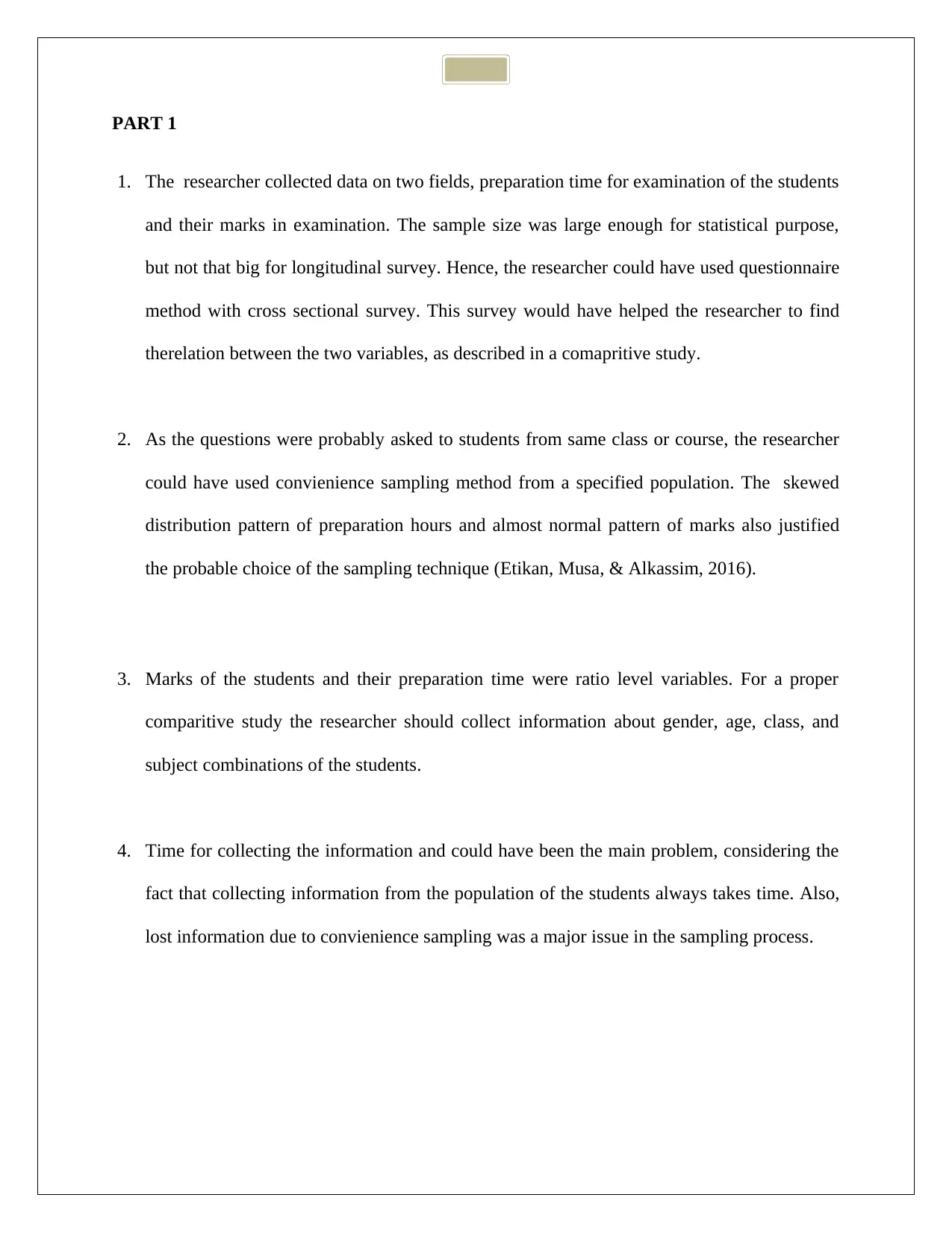
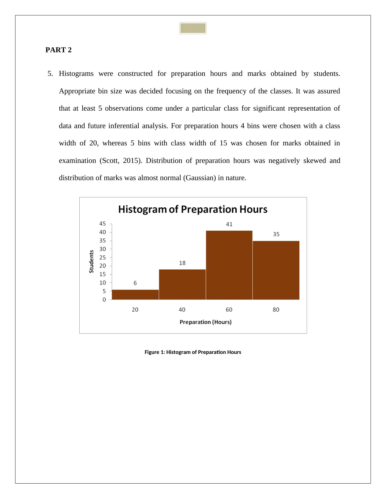
5. Histograms were constructed for preparation hours and marks obtained by students.
Appropriate bin size was decided focusing on the frequency of the classes. It was assured
that at least 5 observations come under a particular class for significant representation of
data and future inferential analysis. For preparation hours 4 bins were chosen with a class
width of 20, whereas 5 bins with class width of 15 was chosen for marks obtained in
examination (Scott, 2015). Distribution of preparation hours was negatively skewed and
distribution of marks was almost normal (Gaussian) in nature.
Figure 1: Histogram of Preparation Hours
You're viewing a preview
Unlock full access by subscribing today!
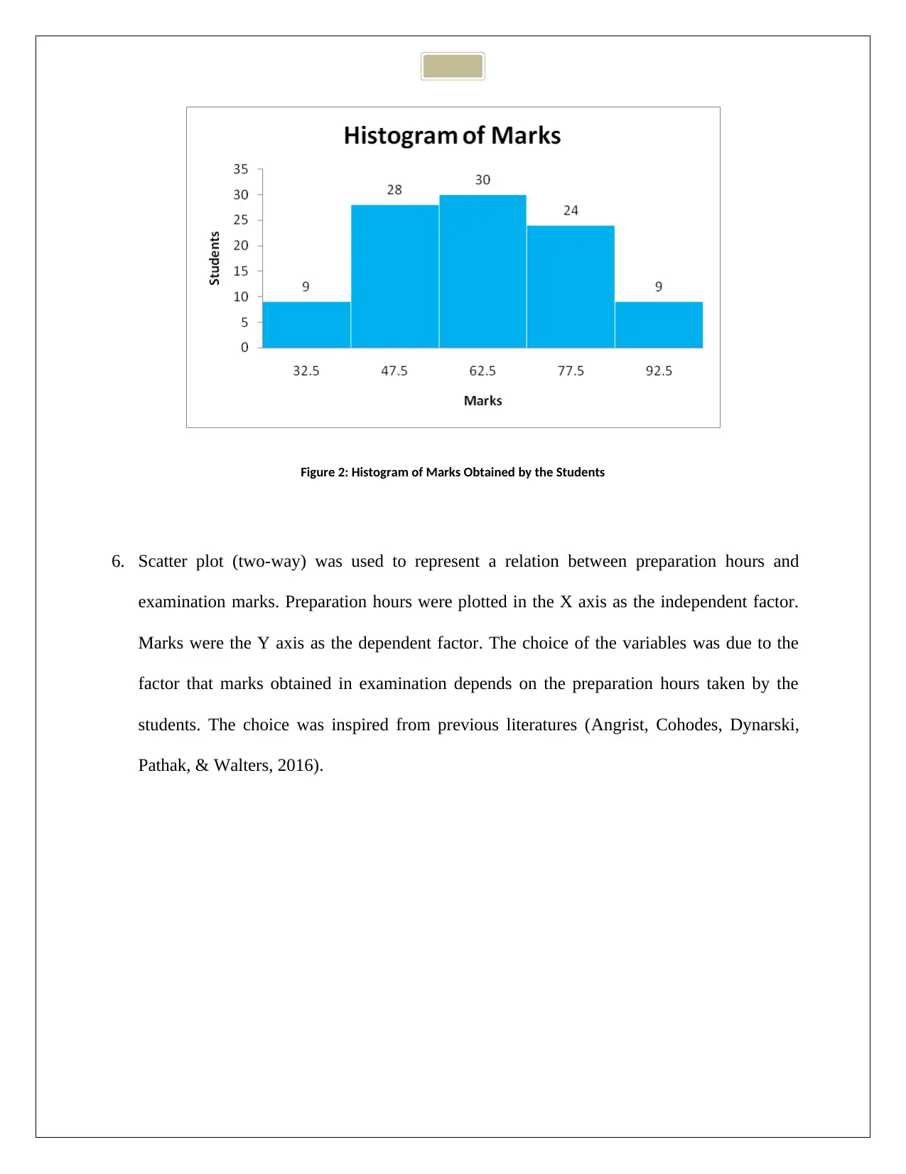
Figure 2: Histogram of Marks Obtained by the Students
6. Scatter plot (two-way) was used to represent a relation between preparation hours and
examination marks. Preparation hours were plotted in the X axis as the independent factor.
Marks were the Y axis as the dependent factor. The choice of the variables was due to the
factor that marks obtained in examination depends on the preparation hours taken by the
students. The choice was inspired from previous literatures (Angrist, Cohodes, Dynarski,
Pathak, & Walters, 2016).
Paraphrase This Document
Need a fresh take? Get an instant paraphrase of this document with our AI Paraphraser
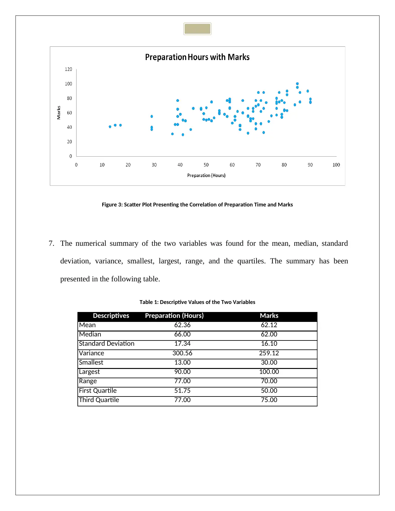
Figure 3: Scatter Plot Presenting the Correlation of Preparation Time and Marks
7. The numerical summary of the two variables was found for the mean, median, standard
deviation, variance, smallest, largest, range, and the quartiles. The summary has been
presented in the following table.
Table 1: Descriptive Values of the Two Variables
Descriptives Preparation (Hours) Marks
Mean 62.36 62.12
Median 66.00 62.00
Standard Deviation 17.34 16.10
Variance 300.56 259.12
Smallest 13.00 30.00
Largest 90.00 100.00
Range 77.00 70.00
First Quartile 51.75 50.00
Third Quartile 77.00 75.00
8. The strength of the relationship of the two variables was assessed by Pearson’s Correlation.
The correlation (R = 0.57) between preparation time and marks obtained was significantly
positive. The trend indicated that marks obtained depended positively on the preparation
time. The association was on the stronger side, and the trend was visible in the scattering of
the data in the scatter plot (Puth, Neuhäuser, & Ruxton, 2014).
9. The confidence interval with 90% confidence was constructed for the population average
time spent on exam preparations. The estimated interval was found as [59.48, 65.24] from
the template spreadsheet on the course website. The t-distribution for unknown sigma was
utilized for the purpose.
10. Hypothesis testing for the assumption of average time spent by student population on
preparation was more than 65 hours (Kim, 2015).
Null hypothesis: H0: ( μ=65 )
Alternate hypothesis H1: ( μ>65 ) Right tail)
Choice was test was t-test, since population standard deviation was not available.
Level of significance was taken as 5%, and therefore, α=0 . 05
Sample mean = x
−
=62 . 36 hours and sample standard deviation = s=17 . 34 hours.
The confidence interval was found as [59.48, 65.24] (from the template Excel spreadsheet).
The test statistic was
t= sample mean− population mean
S tan dard error =62. 36−65
17 .34
√ 100
=−1 .52
(from the t-
Mean sigma unknown spreadsheet) with p-value = 0.0655.
You're viewing a preview
Unlock full access by subscribing today!

At 5% level of significance with 99 degrees of freedom critical t-value (one tail) was
calculated as t = 1.6604.
Hence, the null hypothesis failed to get rejected at 5% level as t cal<tcrit and the p-value was
greater than 0.05. The estimated population mean with 95% confidence for preparation
hours was observed to be within 59.48 hours and 65.24 hours. Hence, the estimated average
preparation time greater than 65.24 hours would have been rejected at 5% level.
11. The linear regression equation was estimated in Excel and the output has been presented in
Table2. The estimated linear equation was found as Marks(Y )=0 .53 *Pr eparation( X )+29. 07 .
The slope of 0.53 (t = 6.88, p< 0.05) of the preparation hours implied a significant linear
relation with marks obtained. The value of the intercept indicated that a student will obtain
approximately 29 marks even without any preparation (preparation time = 0 hour).
Table 2: Regression Model at 5% Level of Significance
Regression Statistics
Multiple R 0.5709
R Square 0.3259
Adjusted R Square 0.3190
Standard Error 13.2837
Observations 100
ANOVA
df SS MS F Significance F
Regression 1 8359.7901 8359.7901 47.3758 0.0000
Residual 98 17292.7699 176.4568
Total 99 25652.5600
Coefficients Standard Error t Stat P-value Lower 95% Upper 95%
Intercept 29.0660 4.9826 5.8335 0.0000 19.1782 38.9538
Preparation (Hours) 0.5301 0.0770 6.8830 0.0000 0.3772 0.6829
12. The coefficient of determination (R-Square) was 0.3259, which indicated that preparation
time (in hours) was able to explain 32.59% variation of marks obtained by the students. The
reason for the low value of R-square could have been the presence of other independent
factors that were not included in the study (Nakagawa, Johnson, & Schielzeth, 2017).
Paraphrase This Document
Need a fresh take? Get an instant paraphrase of this document with our AI Paraphraser
References
Angrist, J. D., Cohodes, S. R., Dynarski, S. M., Pathak, P. A., & Walters, C. R. (2016). Stand
and deliver: Effects of Boston’s charter high schools on college preparation, entry, and
choice. Journal of Labor Economics, 34(2), 275-318.
Etikan, I., Musa, S. A., & Alkassim, R. S. (2016). Comparison of convenience sampling and
purposive sampling. American Journal of Theoretical and Applied Statistics, 5(1), 1-4.
Kim, T. K. (2015). T test as a parametric statistic. Korean journal of anesthesiology, 68(6), 540-
546.
Nakagawa, S., Johnson, P. C., & Schielzeth, H. (2017). The coefficient of determination R2 and
intra-class correlation coefficient from generalized linear mixed-effects models revisited
and expanded. Journal of the Royal Society Interface, 14(134), 20170213.
Puth, M. T., Neuhäuser, M., & Ruxton, G. D. (2014). Effective use of Pearson's product–moment
correlation coefficient. Animal Behaviour, 93, 183-189.
Scott, D. W. (2015). Multivariate density estimation: theory, practice, and visualization. John
Wiley & Sons.
1 out of 8
Related Documents
Your All-in-One AI-Powered Toolkit for Academic Success.
+13062052269
info@desklib.com
Available 24*7 on WhatsApp / Email
![[object Object]](/_next/static/media/star-bottom.7253800d.svg)
Unlock your academic potential
© 2024 | Zucol Services PVT LTD | All rights reserved.


