Business Decision Making

This article discusses business decision making with a focus on GPA, smoker, and child rank. It includes descriptive statistics of these variables and a comparison of the population of students living in urban areas in 2017 and 2018. Additionally, it covers a t-Test analysis of the average rent in two suburbs.

Running head: BUSINESS DECISION MAKING 1
Business Decision Making
Name
Student

BUSINESS DECISION MAKING 2
Business Decision Making
Q1
1. The population of University A to be studied is 280 students.
2. GPA, Smoker and the child rank in the family
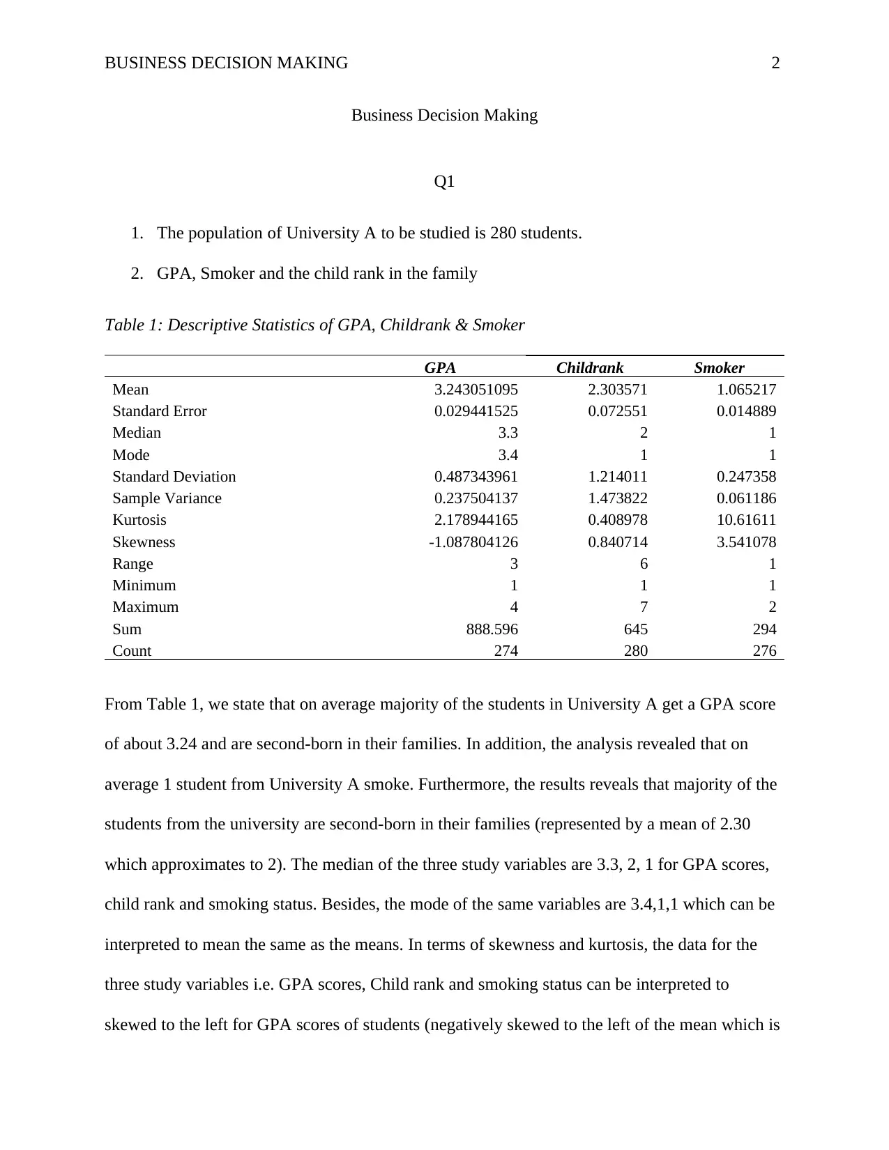
Table 1: Descriptive Statistics of GPA, Childrank & Smoker
GPA Childrank Smoker
Mean 3.243051095 2.303571 1.065217
Standard Error 0.029441525 0.072551 0.014889
Median 3.3 2 1
Mode 3.4 1 1
Standard Deviation 0.487343961 1.214011 0.247358
Sample Variance 0.237504137 1.473822 0.061186
Kurtosis 2.178944165 0.408978 10.61611
Skewness -1.087804126 0.840714 3.541078
Range 3 6 1
Minimum 1 1 1
Maximum 4 7 2
Sum 888.596 645 294
Count 274 280 276
From Table 1, we state that on average majority of the students in University A get a GPA score
of about 3.24 and are second-born in their families. In addition, the analysis revealed that on
average 1 student from University A smoke. Furthermore, the results reveals that majority of the
students from the university are second-born in their families (represented by a mean of 2.30
which approximates to 2). The median of the three study variables are 3.3, 2, 1 for GPA scores,
child rank and smoking status. Besides, the mode of the same variables are 3.4,1,1 which can be
interpreted to mean the same as the means. In terms of skewness and kurtosis, the data for the
three study variables i.e. GPA scores, Child rank and smoking status can be interpreted to
skewed to the left for GPA scores of students (negatively skewed to the left of the mean which is

BUSINESS DECISION MAKING 3
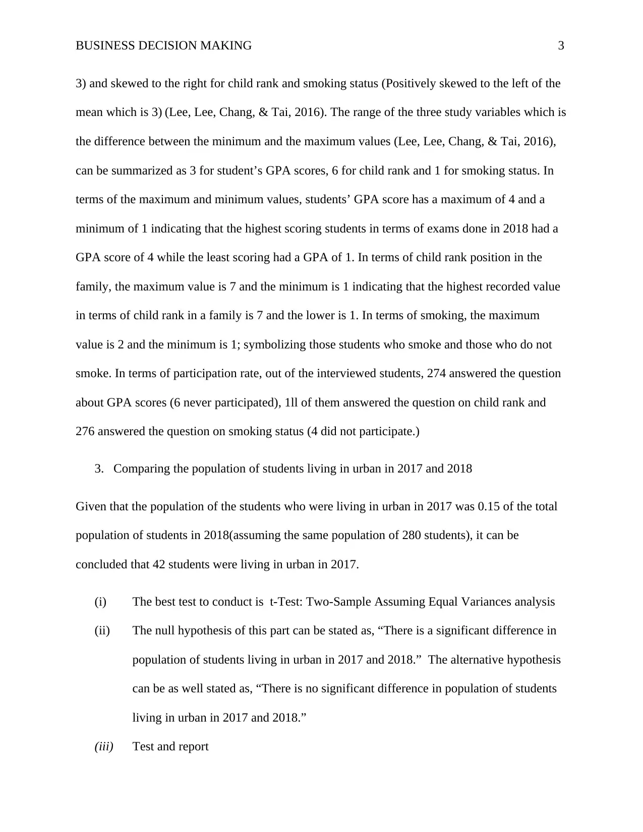
3) and skewed to the right for child rank and smoking status (Positively skewed to the left of the
mean which is 3) (Lee, Lee, Chang, & Tai, 2016). The range of the three study variables which is
the difference between the minimum and the maximum values (Lee, Lee, Chang, & Tai, 2016),
can be summarized as 3 for student’s GPA scores, 6 for child rank and 1 for smoking status. In
terms of the maximum and minimum values, students’ GPA score has a maximum of 4 and a
minimum of 1 indicating that the highest scoring students in terms of exams done in 2018 had a
GPA score of 4 while the least scoring had a GPA of 1. In terms of child rank position in the
family, the maximum value is 7 and the minimum is 1 indicating that the highest recorded value
in terms of child rank in a family is 7 and the lower is 1. In terms of smoking, the maximum
value is 2 and the minimum is 1; symbolizing those students who smoke and those who do not
smoke. In terms of participation rate, out of the interviewed students, 274 answered the question
about GPA scores (6 never participated), 1ll of them answered the question on child rank and
276 answered the question on smoking status (4 did not participate.)
3. Comparing the population of students living in urban in 2017 and 2018
Given that the population of the students who were living in urban in 2017 was 0.15 of the total
population of students in 2018(assuming the same population of 280 students), it can be
concluded that 42 students were living in urban in 2017.
(i) The best test to conduct is t-Test: Two-Sample Assuming Equal Variances analysis
(ii) The null hypothesis of this part can be stated as, “There is a significant difference in
population of students living in urban in 2017 and 2018.” The alternative hypothesis
can be as well stated as, “There is no significant difference in population of students
living in urban in 2017 and 2018.”
(iii) Test and report

BUSINESS DECISION MAKING 4
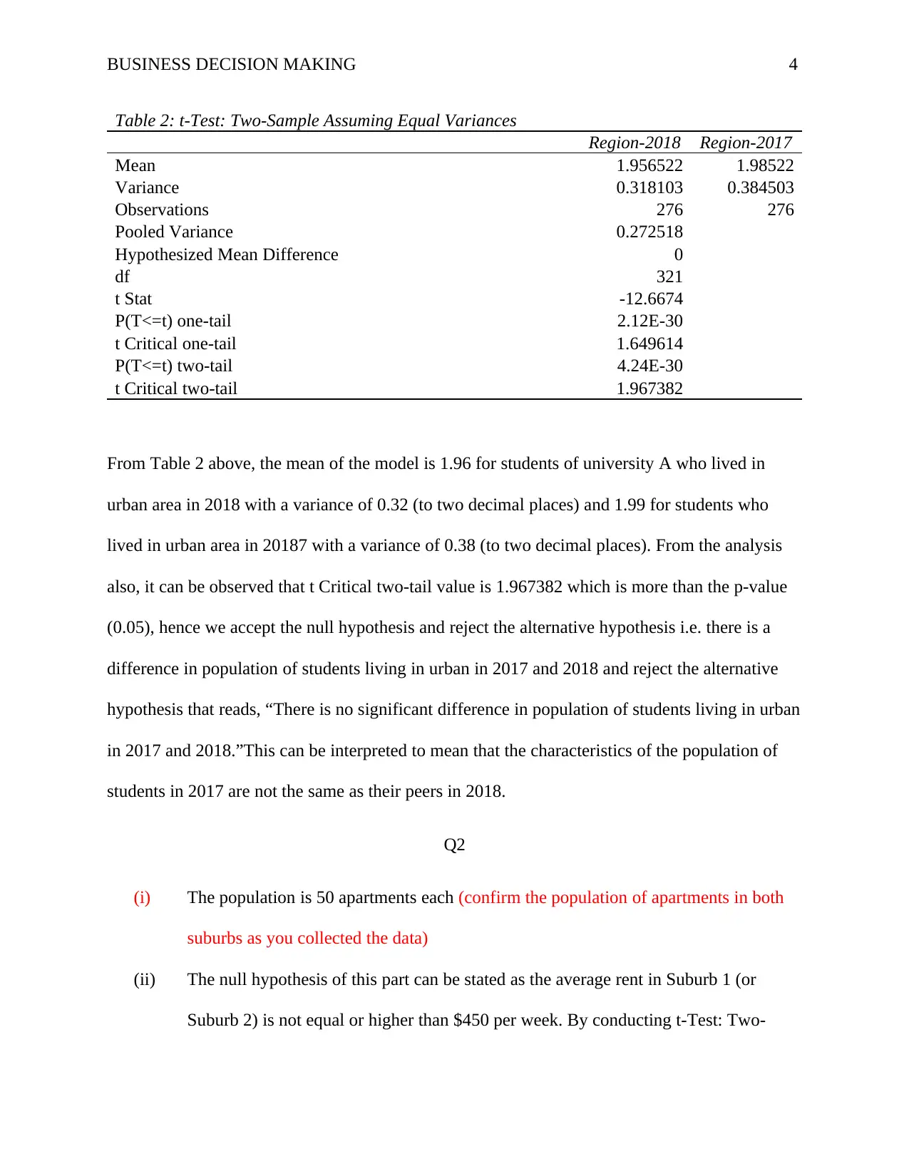
Table 2: t-Test: Two-Sample Assuming Equal Variances
Region-2018 Region-2017
Mean 1.956522 1.98522
Variance 0.318103 0.384503
Observations 276 276
Pooled Variance 0.272518
Hypothesized Mean Difference 0
df 321
t Stat -12.6674
P(T<=t) one-tail 2.12E-30
t Critical one-tail 1.649614
P(T<=t) two-tail 4.24E-30
t Critical two-tail 1.967382
From Table 2 above, the mean of the model is 1.96 for students of university A who lived in
urban area in 2018 with a variance of 0.32 (to two decimal places) and 1.99 for students who
lived in urban area in 20187 with a variance of 0.38 (to two decimal places). From the analysis
also, it can be observed that t Critical two-tail value is 1.967382 which is more than the p-value
(0.05), hence we accept the null hypothesis and reject the alternative hypothesis i.e. there is a
difference in population of students living in urban in 2017 and 2018 and reject the alternative
hypothesis that reads, “There is no significant difference in population of students living in urban
in 2017 and 2018.”This can be interpreted to mean that the characteristics of the population of
students in 2017 are not the same as their peers in 2018.
Q2
(i) The population is 50 apartments each (confirm the population of apartments in both
suburbs as you collected the data)
(ii) The null hypothesis of this part can be stated as the average rent in Suburb 1 (or
Suburb 2) is not equal or higher than $450 per week. By conducting t-Test: Two-

BUSINESS DECISION MAKING 5
Sample Assuming Equal Variance analysis, the table below with some key statistics
is obtained.

BUSINESS DECISION MAKING 6
Table 2: t-Test: Two-Sample Assuming Equal Variances
St MARYS Penrith NSW
Mean 335.8 377.6
Variance 1816.694 4059.429
Observations 50 50
Pooled Variance 2938.061
Hypothesized Mean Difference 450
df 98
t Stat -45.3658
P(T<=t) one-tail 6.84E-68
t Critical one-tail 1.660551
P(T<=t) two-tail 1.37E-67
t Critical two-tail 1.984467
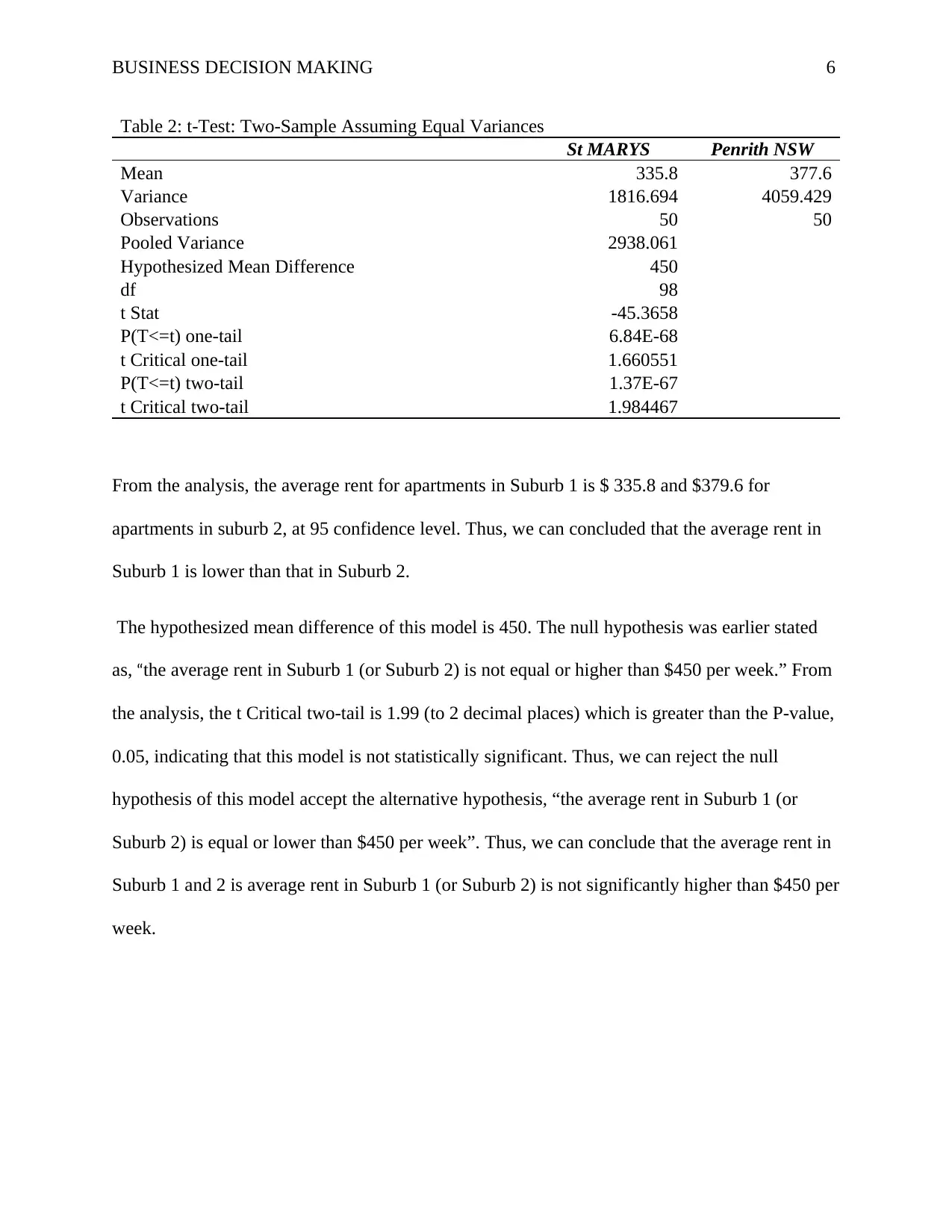
From the analysis, the average rent for apartments in Suburb 1 is $ 335.8 and $379.6 for
apartments in suburb 2, at 95 confidence level. Thus, we can concluded that the average rent in
Suburb 1 is lower than that in Suburb 2.
The hypothesized mean difference of this model is 450. The null hypothesis was earlier stated
as, “the average rent in Suburb 1 (or Suburb 2) is not equal or higher than $450 per week.” From
the analysis, the t Critical two-tail is 1.99 (to 2 decimal places) which is greater than the P-value,
0.05, indicating that this model is not statistically significant. Thus, we can reject the null
hypothesis of this model accept the alternative hypothesis, “the average rent in Suburb 1 (or
Suburb 2) is equal or lower than $450 per week”. Thus, we can conclude that the average rent in
Suburb 1 and 2 is average rent in Suburb 1 (or Suburb 2) is not significantly higher than $450 per
week.

BUSINESS DECISION MAKING 7
References
Lee, C., Lee, J., Chang, J., & Tai, T. (2016). Professional Techniques Used in Excel and Excel
VBA Techniques. Essentials of Excel, Excel VBA, SAS and Minitab for Statistical and
Financial Analyses, 7(4), 763-800. doi:10.1007/978-3-319-38867-0_24
Lee, C., Lee, J., Chang, J., & Tai, T. (2016). Statistical Decision Theory. Essentials of Excel,
Excel VBA, SAS and Minitab for Statistical and Financial Analyses, 9(2), 685-698.
doi:10.1007/978-3-319-38867-0_21