ANOVA and Regression Analysis

The provided assignment focuses on analyzing data using both ANOVA (Analysis of Variance) and regression techniques. The results are presented in two tables: Table 42 shows the ANOVA computation with degrees of freedom (df), sum of squares (SS), mean squares (MS), F-statistic, and significance level (p-value). Table 43 presents a coefficient table for the regression model, including coefficients, standard errors, t-statistics, p-values, and confidence intervals for each predictor variable.

BUSINESS STATISTICS

TABLE OF CONTENTS
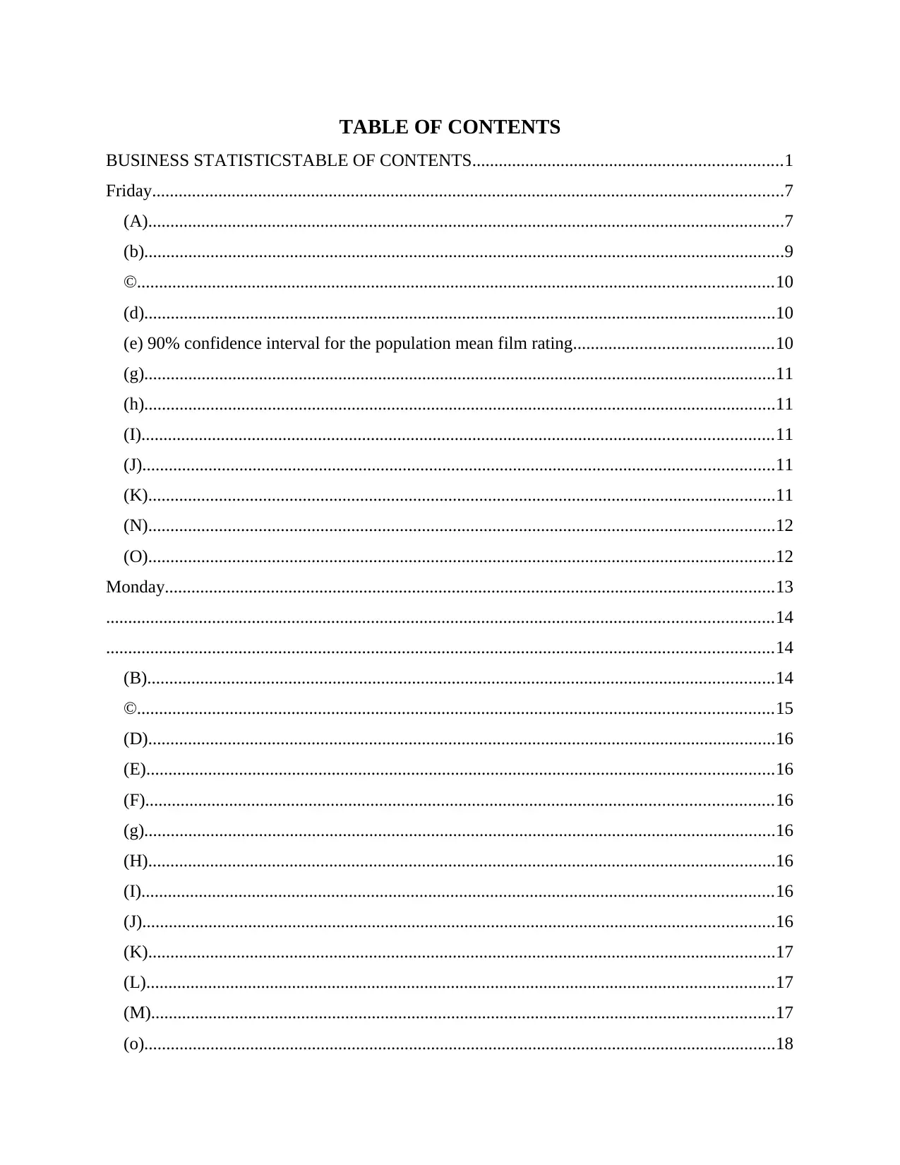
BUSINESS STATISTICSTABLE OF CONTENTS......................................................................1
Friday...............................................................................................................................................7
(A)................................................................................................................................................7
(b).................................................................................................................................................9
©................................................................................................................................................10
(d)...............................................................................................................................................10
(e) 90% confidence interval for the population mean film rating.............................................10
(g)...............................................................................................................................................11
(h)...............................................................................................................................................11
(I)...............................................................................................................................................11
(J)...............................................................................................................................................11
(K)..............................................................................................................................................11
(N)..............................................................................................................................................12
(O)..............................................................................................................................................12
Monday..........................................................................................................................................13
.......................................................................................................................................................14
.......................................................................................................................................................14
(B)..............................................................................................................................................14
©................................................................................................................................................15
(D)..............................................................................................................................................16
(E)..............................................................................................................................................16
(F)..............................................................................................................................................16
(g)...............................................................................................................................................16
(H)..............................................................................................................................................16
(I)...............................................................................................................................................16
(J)...............................................................................................................................................16
(K)..............................................................................................................................................17
(L)..............................................................................................................................................17
(M).............................................................................................................................................17
(o)...............................................................................................................................................18

Thursday........................................................................................................................................19
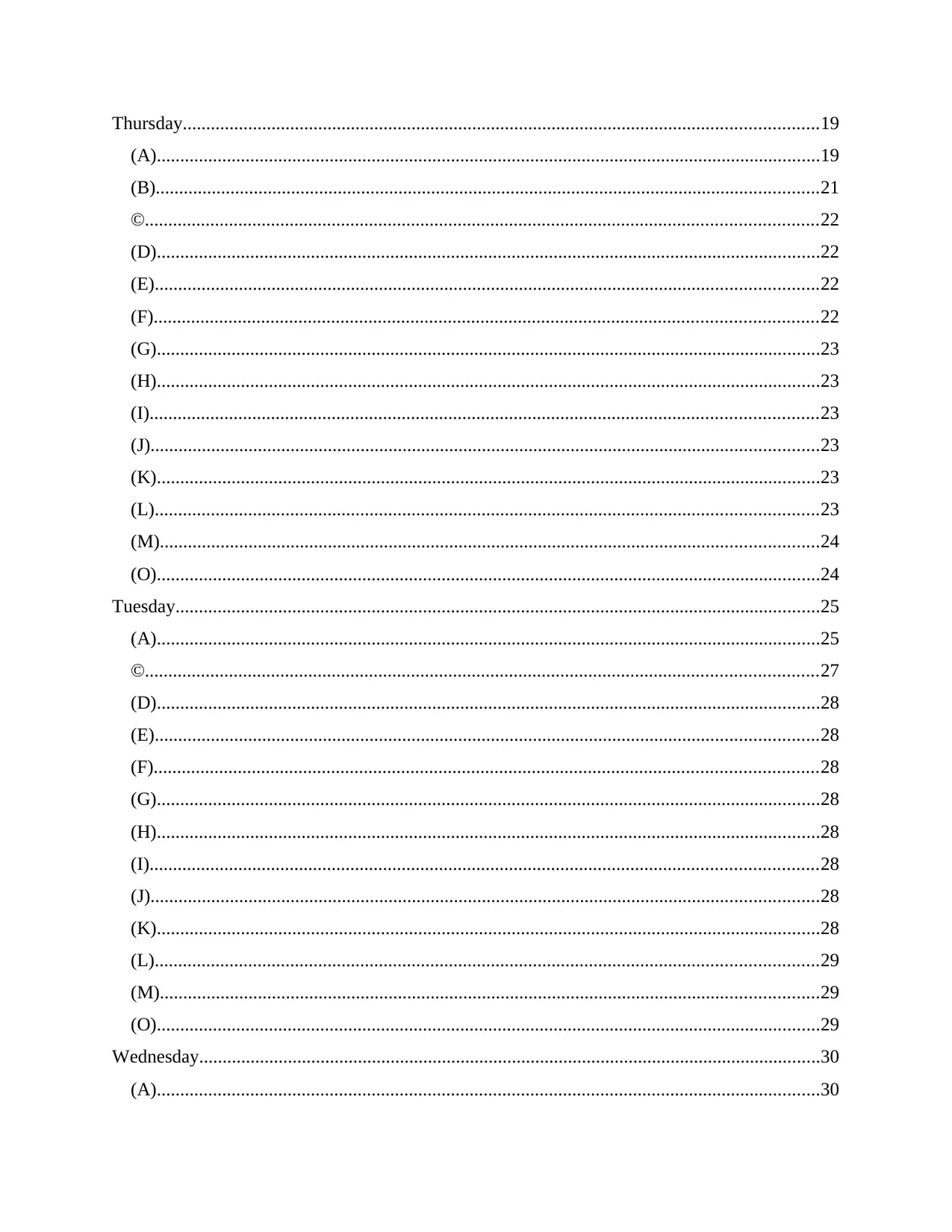
(A)..............................................................................................................................................19
(B)..............................................................................................................................................21
©................................................................................................................................................22
(D)..............................................................................................................................................22
(E)..............................................................................................................................................22
(F)..............................................................................................................................................22
(G)..............................................................................................................................................23
(H)..............................................................................................................................................23
(I)...............................................................................................................................................23
(J)...............................................................................................................................................23
(K)..............................................................................................................................................23
(L)..............................................................................................................................................23
(M).............................................................................................................................................24
(O)..............................................................................................................................................24
Tuesday..........................................................................................................................................25
(A)..............................................................................................................................................25
©................................................................................................................................................27
(D)..............................................................................................................................................28
(E)..............................................................................................................................................28
(F)..............................................................................................................................................28
(G)..............................................................................................................................................28
(H)..............................................................................................................................................28
(I)...............................................................................................................................................28
(J)...............................................................................................................................................28
(K)..............................................................................................................................................28
(L)..............................................................................................................................................29
(M).............................................................................................................................................29
(O)..............................................................................................................................................29
Wednesday.....................................................................................................................................30
(A)..............................................................................................................................................30

(B)..............................................................................................................................................32
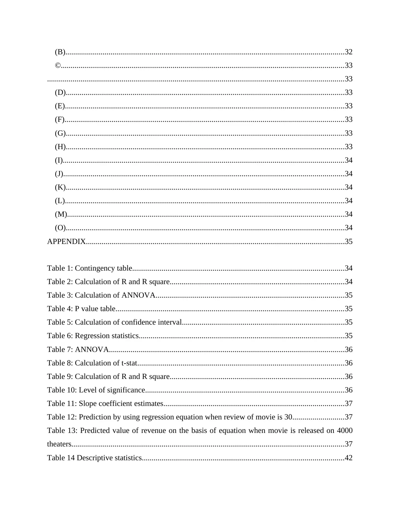
©................................................................................................................................................33
.......................................................................................................................................................33
(D)..............................................................................................................................................33
(E)..............................................................................................................................................33
(F)..............................................................................................................................................33
(G)..............................................................................................................................................33
(H)..............................................................................................................................................33
(I)...............................................................................................................................................34
(J)...............................................................................................................................................34
(K)..............................................................................................................................................34
(L)..............................................................................................................................................34
(M).............................................................................................................................................34
(O)..............................................................................................................................................34
APPENDIX....................................................................................................................................35
Table 1: Contingency table............................................................................................................34
Table 2: Calculation of R and R square.........................................................................................34
Table 3: Calculation of ANNOVA................................................................................................35
Table 4: P value table....................................................................................................................35
Table 5: Calculation of confidence interval...................................................................................35
Table 6: Regression statistics.........................................................................................................35
Table 7: ANNOVA........................................................................................................................36
Table 8: Calculation of t-stat.........................................................................................................36
Table 9: Calculation of R and R square.........................................................................................36
Table 10: Level of significance.....................................................................................................36
Table 11: Slope coefficient estimates............................................................................................37
Table 12: Prediction by using regression equation when review of movie is 30..........................37
Table 13: Predicted value of revenue on the basis of equation when movie is released on 4000
theaters...........................................................................................................................................37
Table 14 Descriptive statistics.......................................................................................................42

Table 15 Contingency table...........................................................................................................42
Table 16 Table of regression.........................................................................................................43
Table 17 Table of ANNOVA........................................................................................................43
Table 18 Table of coefficients.......................................................................................................43
Table 19 Range of bedrooms at 99% confidence interval.............................................................44
Table 20 Computation of regression statistics...............................................................................44
Table 21Calculation of ANNOVA................................................................................................44
Table 22 Coefficients of variables.................................................................................................44
Table 23 Statistics of regression for G part of Thursday...............................................................45
Table 24 Table of ANNOVA........................................................................................................45
Table 25 Computation of coefficients...........................................................................................45
Table 26 Contingency table...........................................................................................................47
Table 27 Calculation of regression................................................................................................47
Table 28 Computation of ANNOVA.............................................................................................47
Table 29 Calculation of coefficient...............................................................................................48
Table 30 Range at 90% confidence interval..................................................................................48
Table 31 Summary statistics of one way ANNOVA.....................................................................48
Table 32 Variation between and within groups.............................................................................48
Table 33 Regression statistics........................................................................................................49
Table 34 ANNOVA table..............................................................................................................49
Table 35 Coefficient table.............................................................................................................49
Table 36 Table of regression.........................................................................................................50
Table 37ANNOVA table...............................................................................................................50
Table 38 Calculation of coefficient...............................................................................................50
Table 39 95% Confidence interval................................................................................................50
Table 40 One way ANNOVA........................................................................................................51
Table 41Calculation of regression.................................................................................................51
Table 42 Computation of ANNOVA.............................................................................................52
Table 43 Coefficient table..........................................................................................................................52
Figure 1: Shape of Theater..............................................................................................................9

Figure 2: Shape of Metacritic..........................................................................................................9
Figure 3: Shape of gross................................................................................................................10
Figure 4: Number of theater..........................................................................................................10
Figure 5: Box and Whisker plot.....................................................................................................11
Figure 6 Chart on salary................................................................................................................14
Figure 7 Chart on satisfaction........................................................................................................15
Figure 8 Chart on ATAR...............................................................................................................15
Figure 9Chart on Satisfaction........................................................................................................16
Figure 10 Box and Whisker chart..................................................................................................16
Figure 11 Regression equation......................................................................................................18
Figure 12Chart on number of bedrooms........................................................................................20
Figure 13Chart on price of homes.................................................................................................21
Figure 14 Chart on land area.........................................................................................................21
Figure 15 Chart on mile distance...................................................................................................22
Figure 16 Distance graph...............................................................................................................22
Figure 17 Box and Whisker chart..................................................................................................23
Figure 18 Chart on battery score...................................................................................................26
Figure 19 Chart on pic density.......................................................................................................27
Figure 20 Chart on score................................................................................................................27
Figure 21 Chart on review score....................................................................................................28
Figure 22 Box and whisker chart...................................................................................................28
Figure 23Regression equation.......................................................................................................30
Figure 24 Price of cars...................................................................................................................31
Figure 25 Power capacity of car....................................................................................................32
Figure 26 Weight of cars...............................................................................................................32
Figure 27 Fuel efficiency of car.....................................................................................................33
Figure 28 Distribution of fuel........................................................................................................33
Figure 29Box and Whisker plot.....................................................................................................34
Figure 30 Regression equation......................................................................................................35
Figure 31Contingency table...........................................................................................................40
Figure 32 Regression table............................................................................................................40

Figure 33 ANNOVA table.............................................................................................................40
Figure 34 Coefficient table............................................................................................................41
Figure 35 95% Confidence interval...............................................................................................41
Figure 36 Statistics of regression...................................................................................................41
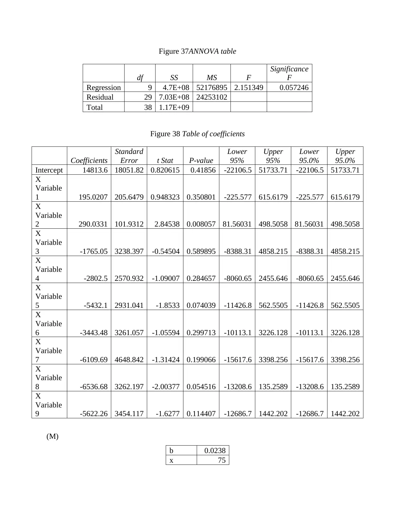
Figure 37ANNOVA table..............................................................................................................42
Figure 38 Table of coefficients......................................................................................................42

Friday
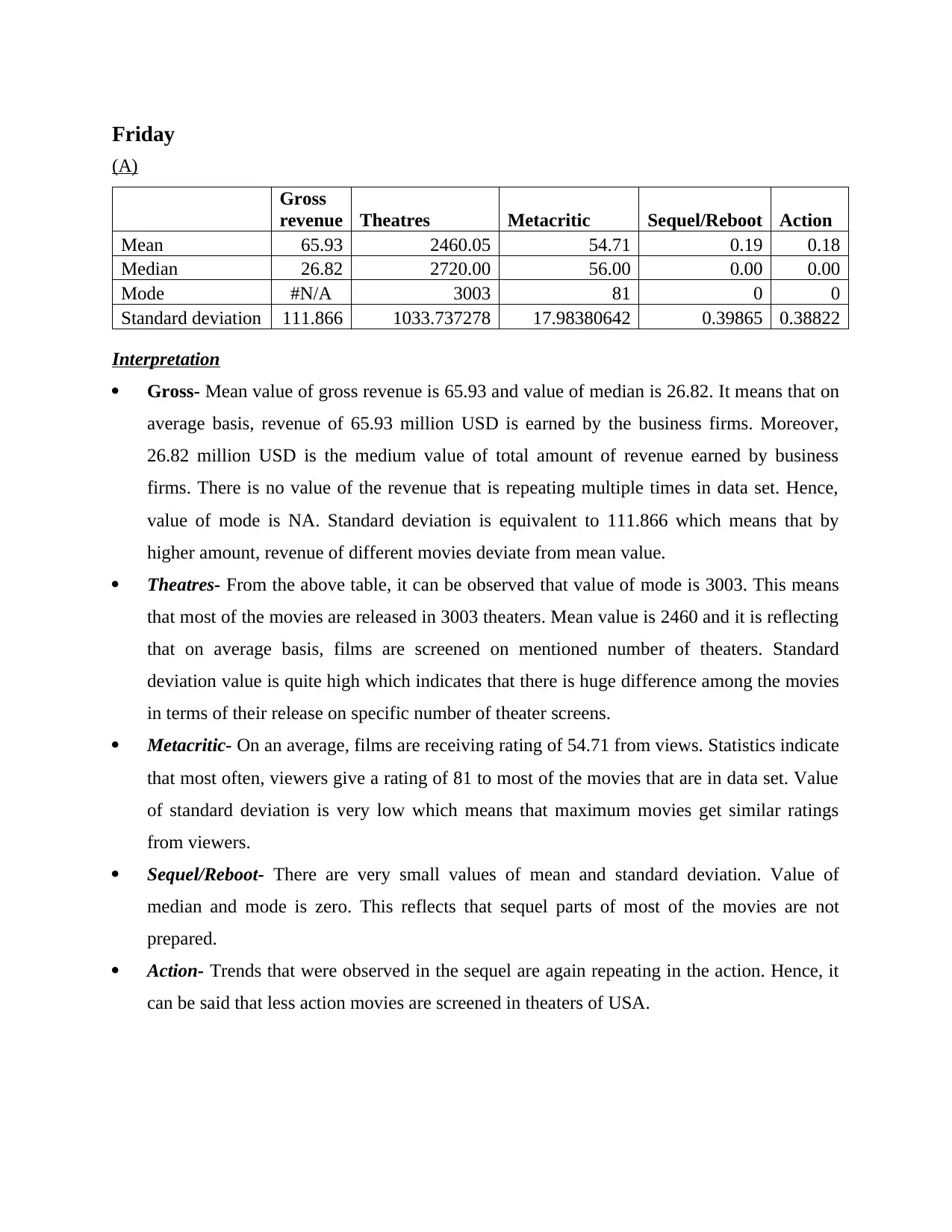
(A)
Gross
revenue Theatres Metacritic Sequel/Reboot Action
Mean 65.93 2460.05 54.71 0.19 0.18
Median 26.82 2720.00 56.00 0.00 0.00
Mode #N/A 3003 81 0 0
Standard deviation 111.866 1033.737278 17.98380642 0.39865 0.38822
Interpretation
 Gross- Mean value of gross revenue is 65.93 and value of median is 26.82. It means that on
average basis, revenue of 65.93 million USD is earned by the business firms. Moreover,
26.82 million USD is the medium value of total amount of revenue earned by business
firms. There is no value of the revenue that is repeating multiple times in data set. Hence,
value of mode is NA. Standard deviation is equivalent to 111.866 which means that by
higher amount, revenue of different movies deviate from mean value.
 Theatres- From the above table, it can be observed that value of mode is 3003. This means
that most of the movies are released in 3003 theaters. Mean value is 2460 and it is reflecting
that on average basis, films are screened on mentioned number of theaters. Standard
deviation value is quite high which indicates that there is huge difference among the movies
in terms of their release on specific number of theater screens.
 Metacritic- On an average, films are receiving rating of 54.71 from views. Statistics indicate
that most often, viewers give a rating of 81 to most of the movies that are in data set. Value
of standard deviation is very low which means that maximum movies get similar ratings
from viewers.
 Sequel/Reboot- There are very small values of mean and standard deviation. Value of
median and mode is zero. This reflects that sequel parts of most of the movies are not
prepared.
 Action- Trends that were observed in the sequel are again repeating in the action. Hence, it
can be said that less action movies are screened in theaters of USA.

Figure 1: Shape of Theater
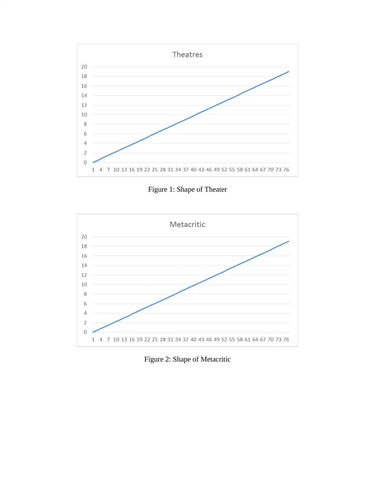
Figure 2: Shape of Metacritic

Figure 3: Shape of gross
(b)
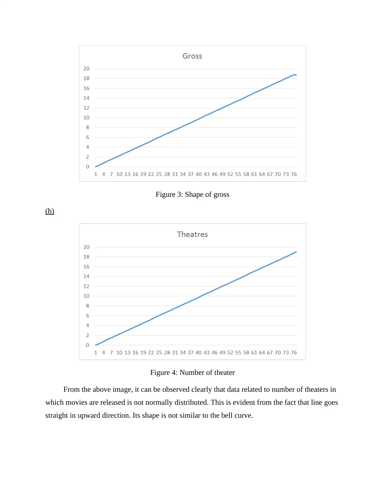
Figure 4: Number of theater
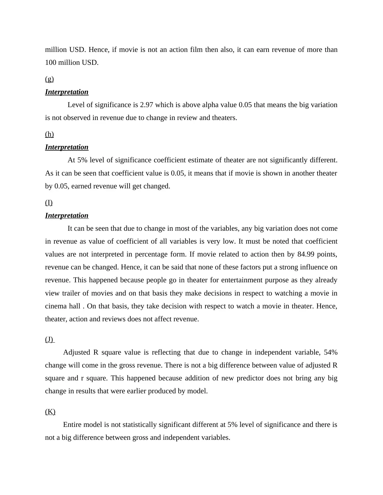
From the above image, it can be observed clearly that data related to number of theaters in
which movies are released is not normally distributed. This is evident from the fact that line goes
straight in upward direction. Its shape is not similar to the bell curve.

©
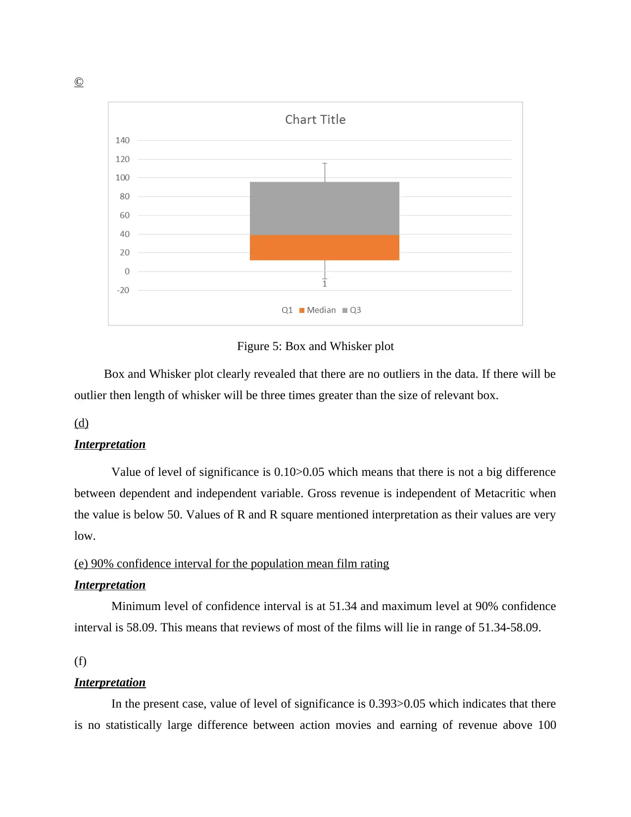
Figure 5: Box and Whisker plot
Box and Whisker plot clearly revealed that there are no outliers in the data. If there will be
outlier then length of whisker will be three times greater than the size of relevant box.
(d)
Interpretation
Value of level of significance is 0.10>0.05 which means that there is not a big difference
between dependent and independent variable. Gross revenue is independent of Metacritic when
the value is below 50. Values of R and R square mentioned interpretation as their values are very
low.
(e) 90% confidence interval for the population mean film rating
Interpretation
Minimum level of confidence interval is at 51.34 and maximum level at 90% confidence
interval is 58.09. This means that reviews of most of the films will lie in range of 51.34-58.09.
(f)
Interpretation
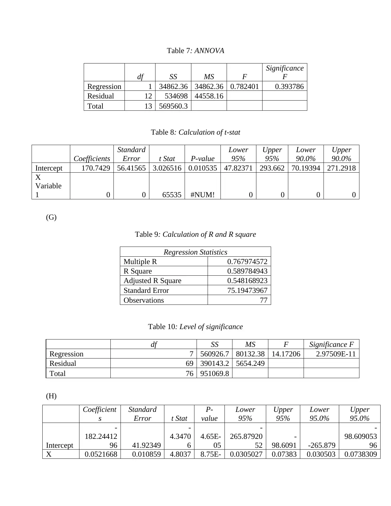
In the present case, value of level of significance is 0.393>0.05 which indicates that there
is no statistically large difference between action movies and earning of revenue above 100

million USD. Hence, if movie is not an action film then also, it can earn revenue of more than
100 million USD.
(g)
Interpretation
Level of significance is 2.97 which is above alpha value 0.05 that means the big variation
is not observed in revenue due to change in review and theaters.
(h)
Interpretation
At 5% level of significance coefficient estimate of theater are not significantly different.
As it can be seen that coefficient value is 0.05, it means that if movie is shown in another theater
by 0.05, earned revenue will get changed.
(I)
Interpretation
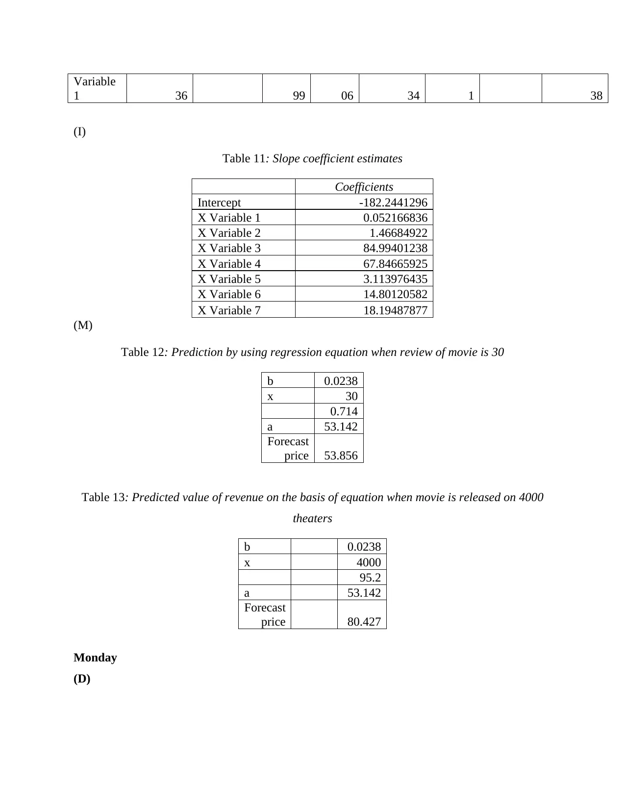
It can be seen that due to change in most of the variables, any big variation does not come
in revenue as value of coefficient of all variables is very low. It must be noted that coefficient
values are not interpreted in percentage form. If movie related to action then by 84.99 points,
revenue can be changed. Hence, it can be said that none of these factors put a strong influence on
revenue. This happened because people go in theater for entertainment purpose as they already
view trailer of movies and on that basis they make decisions in respect to watching a movie in
cinema hall . On that basis, they take decision with respect to watch a movie in theater. Hence,
theater, action and reviews does not affect revenue.
(J)
Adjusted R square value is reflecting that due to change in independent variable, 54%
change will come in the gross revenue. There is not a big difference between value of adjusted R
square and r square. This happened because addition of new predictor does not bring any big
change in results that were earlier produced by model.
(K)
Entire model is not statistically significant different at 5% level of significance and there is
not a big difference between gross and independent variables.

(L)
Trailer is another factor that can influence gross revenue of the film. This is because; on
the basis of trailer, one determines that whether movie is good or bad. Trailer already comes on
internet before release of movie on theater. Hence, it plays a strong role in forming positive or
negative perception about movie among general public.
(M)
Interpretation
If movie is having rating of 30 then it can earn revenue of 53 million USD. Similarly, if
film will be presented in 4000 theaters then revenue of 80.42 million USD can be earned.
(N)
(O)
Rating range of Australia made films is computed. Thus, on basis of estimate can be made
about likely performance of relevant movies.

Monday
(A)
 Salary- None of value is repeated in data set and median value is 43006. Table clearly
reflect that mean is 44,716 and value of standard deviation is 5556. This means that from
salary point of view difference is not observed in comparison to mean in salary of
students that completed BBA.
 Satisfaction- Satisfaction level of students is very high as indicated by mean value of 83.
Value of mode is 83. Apart from this, value of standard deviation is only 4. This, further
provide support to the interpretation made above.
 ATAR- For getting an admission in colleges mean ATAR requirement is 66. Value of
mode is 70 and same of standard deviation is 13. This means that in most of colleges in
order to get admission one have to score between 66-70
 Mean of dummy variables- Mean of dummy variables is zero and this reflect that
majority of universities are not located in specific location.
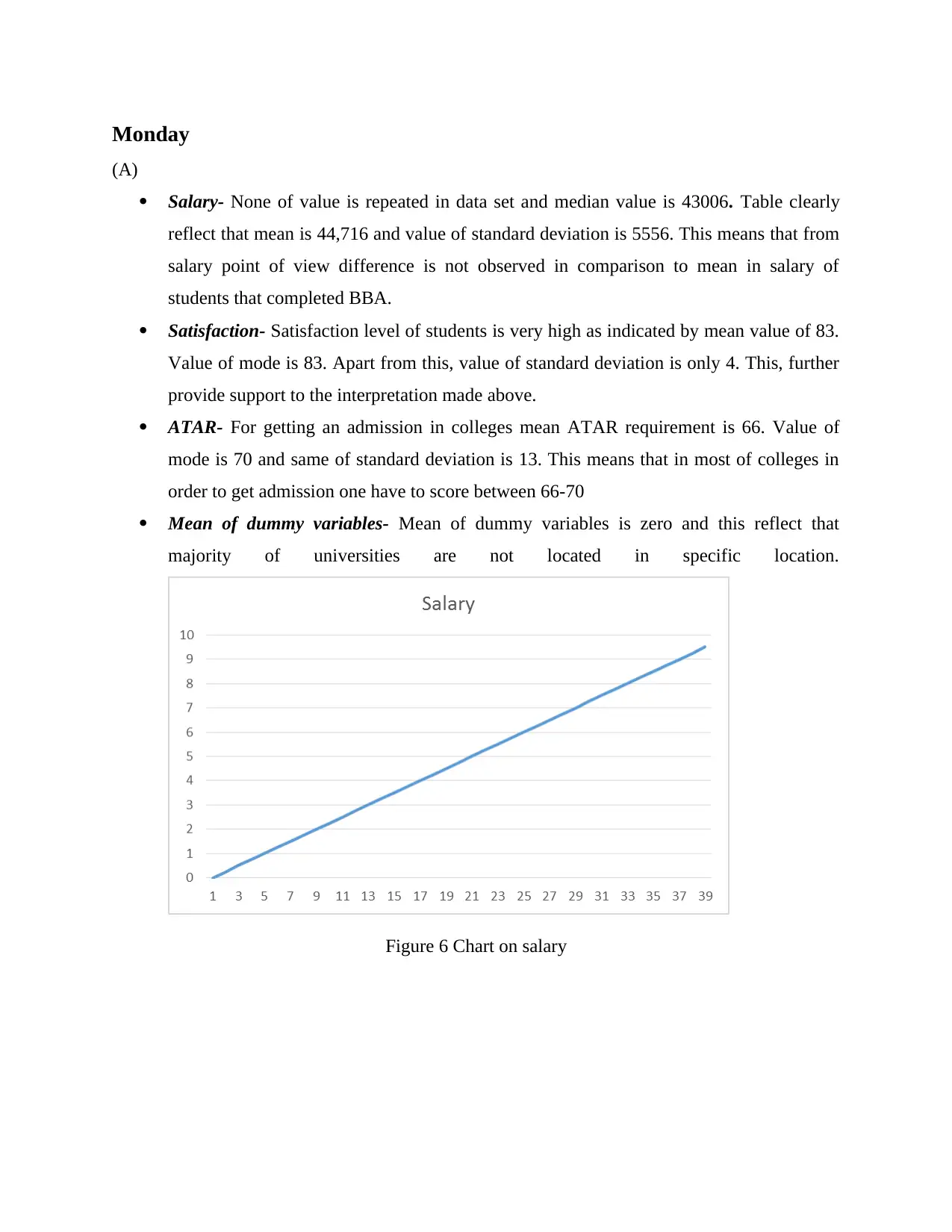
Figure 6 Chart on salary

Figure 7 Chart on satisfaction
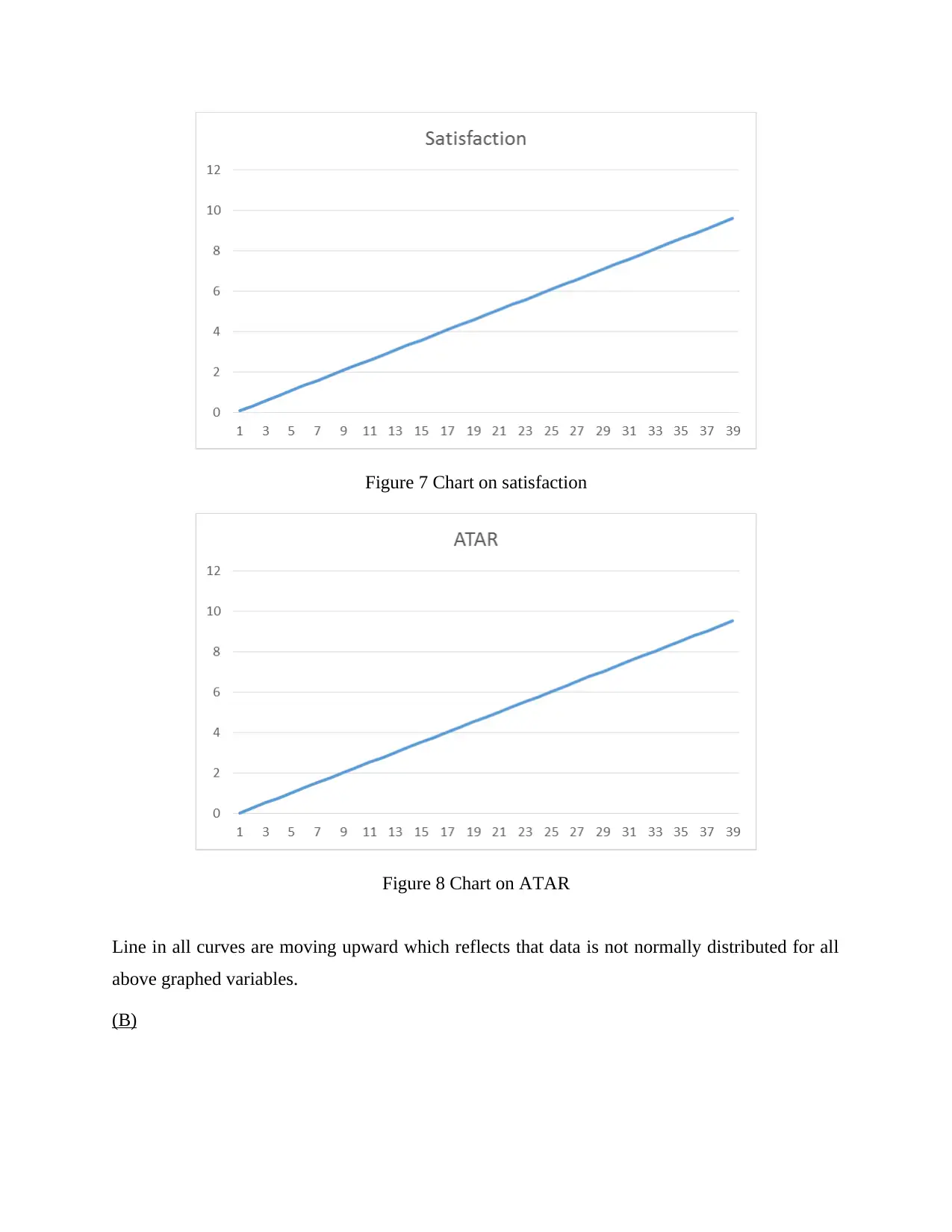
Figure 8 Chart on ATAR
Line in all curves are moving upward which reflects that data is not normally distributed for all
above graphed variables.
(B)

Figure 9Chart on Satisfaction
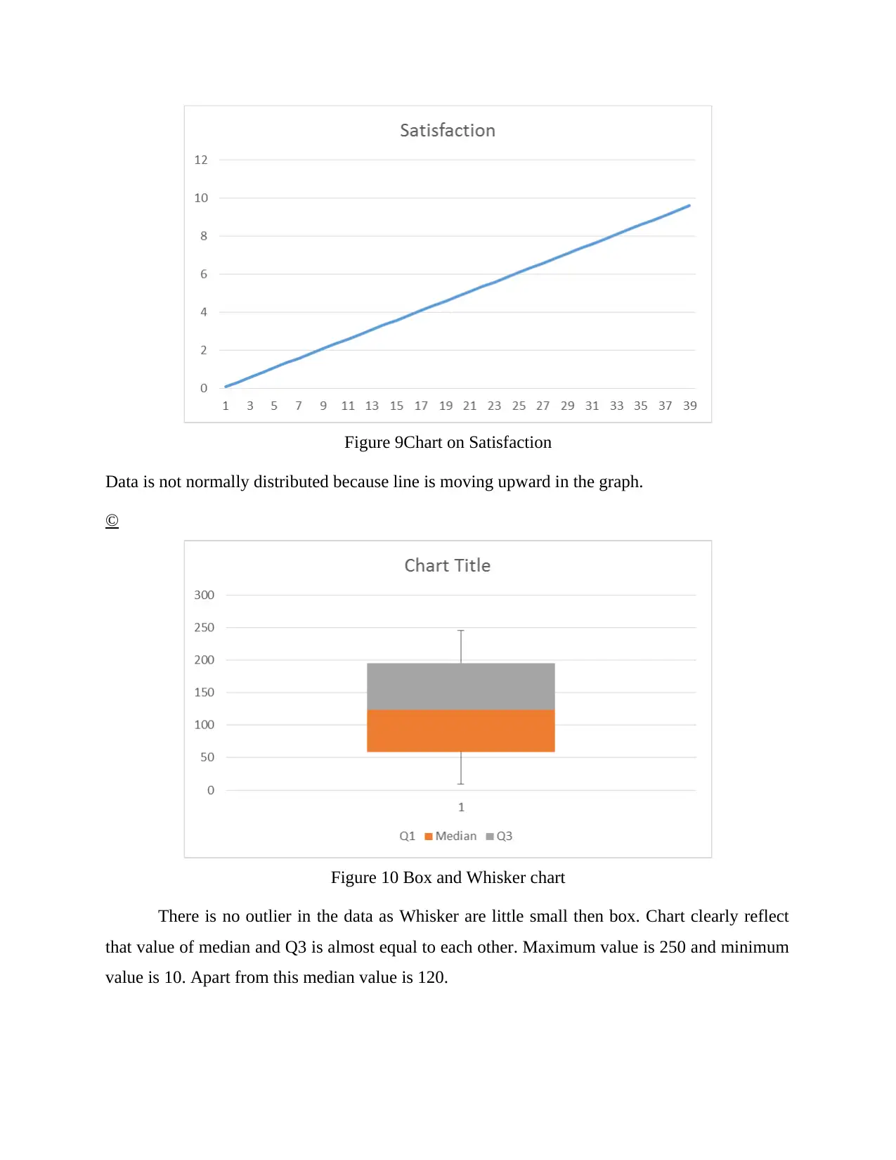
Data is not normally distributed because line is moving upward in the graph.
©
Figure 10 Box and Whisker chart
There is no outlier in the data as Whisker are little small then box. Chart clearly reflect
that value of median and Q3 is almost equal to each other. Maximum value is 250 and minimum
value is 10. Apart from this median value is 120.

(D)
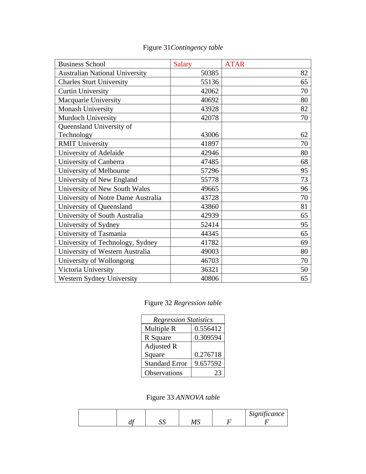
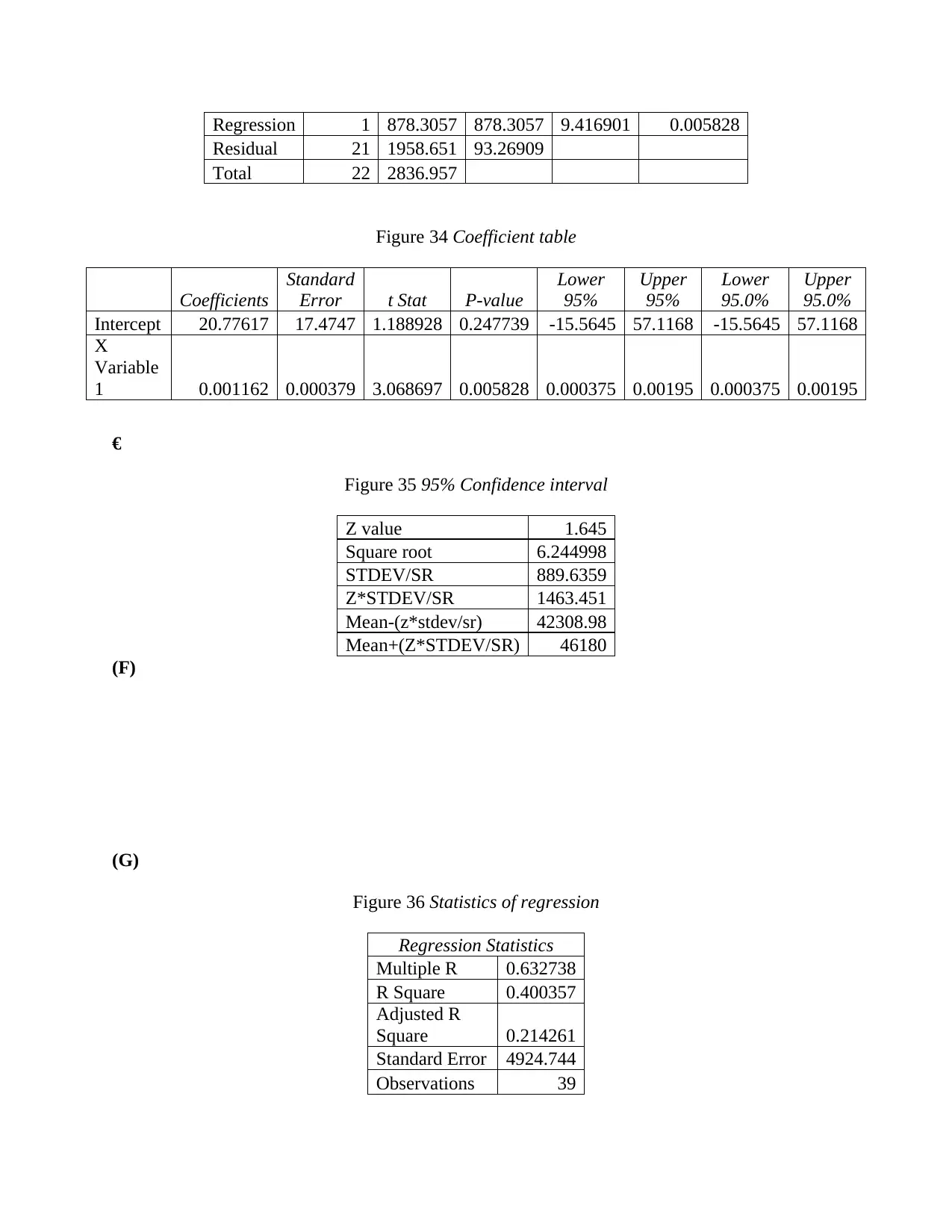
Level of significance is 0.005<0.05 and this reflects that there is significant difference in
the salary and ATAR score. This means that with change in entrance score of ATAR big
variation is observed in student’s salary. There is high probability that average student earn more
than 46,000 when ATAR score exceed 65.
(E)
At 95% confidence interval with mean and standard deviation of 44716 and 5556 salary of
students will remain in range of 42308- 46180.
(F)
Need to be done
(g)
There is statistically significant difference in mean value of salary and other variables. As
value of level of significance is 0.05 which is equal to alpha. Hence, it can be said that with small
change in independent variables moderate variation comes in salary.
(H)
Value of ATAR coefficient is 290 which means that with change in mentioned variable
salary will change by 290 points. It can be said that ATAR put a small impact on salary of
students.
(I)
Coefficient results reflect that if students will be satisfied from graduation program their
salary will increase. In case of dummy variables value of coefficient is negative which means
that if negative changes happen in universities then salary of the students may be low.

(J)
Value of adjusted R square is 0.21 which means that salary of students get changed by
21% with small change in independent variables. There is a moderate difference between values
of R square and Adjusted R square. This happened because addition of new variable in model is
brining moderate change in its results.
(K)
Model is statistically significant at 5% level of significance and it is clear that dependent
variable get changed with change in independent variable.
(L)
Practical training that is given to the students is the factor that greatly influence graduate
salary.
(M)
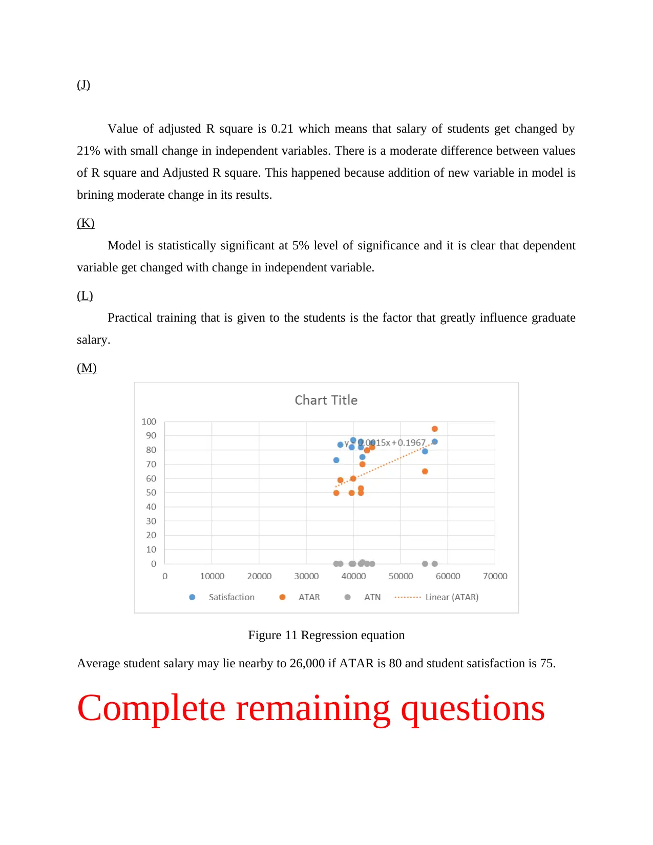
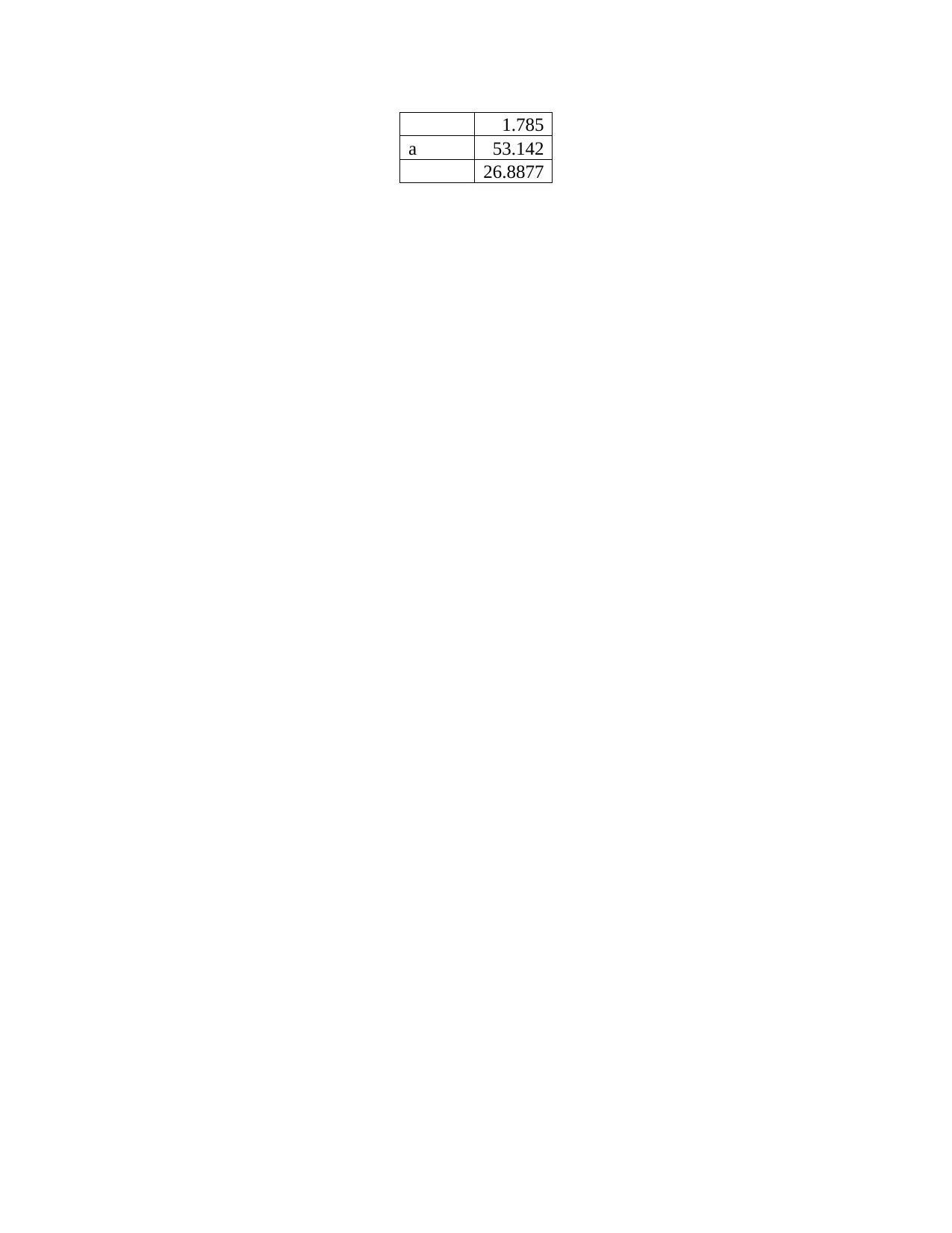
Figure 11 Regression equation
Average student salary may lie nearby to 26,000 if ATAR is 80 and student satisfaction is 75.
Complete remaining questions

(o)
Stratified random sampling method must be used to take appropriate sample for research.

Thursday
(A)
 Price- Most houses are price at 3, 80,000 as indicated by median. On average basis houses
are priced at 5, 84,214. Standard deviation value is high which reflects that there is big
difference in price of various houses.
 Bedroom- In most houses there are three bedrooms as indicated by values of descriptive
statistics tools.
 Land area- Average land are covered by most houses is 803. Standard deviation value is
high which indicate that there is big difference among houses in terms of land are covered by
them. Apart from this, there are number of houses that commonly cover an area of 559 Sq m
as reflected by mode.
 Distance to Melbourne- Average houses that are away from Melbourne have distance of 25
KM from mentioned city. There are number of houses that are located 16 KM away from
Melbourne. Standard deviation is moderate which means that comparatively there is medium
distance of houses from relevant city.
 Dummy variables- Mean value of dummy variables is very small which means that large
number of houses that are in the data set are not collectively sold in specific year.
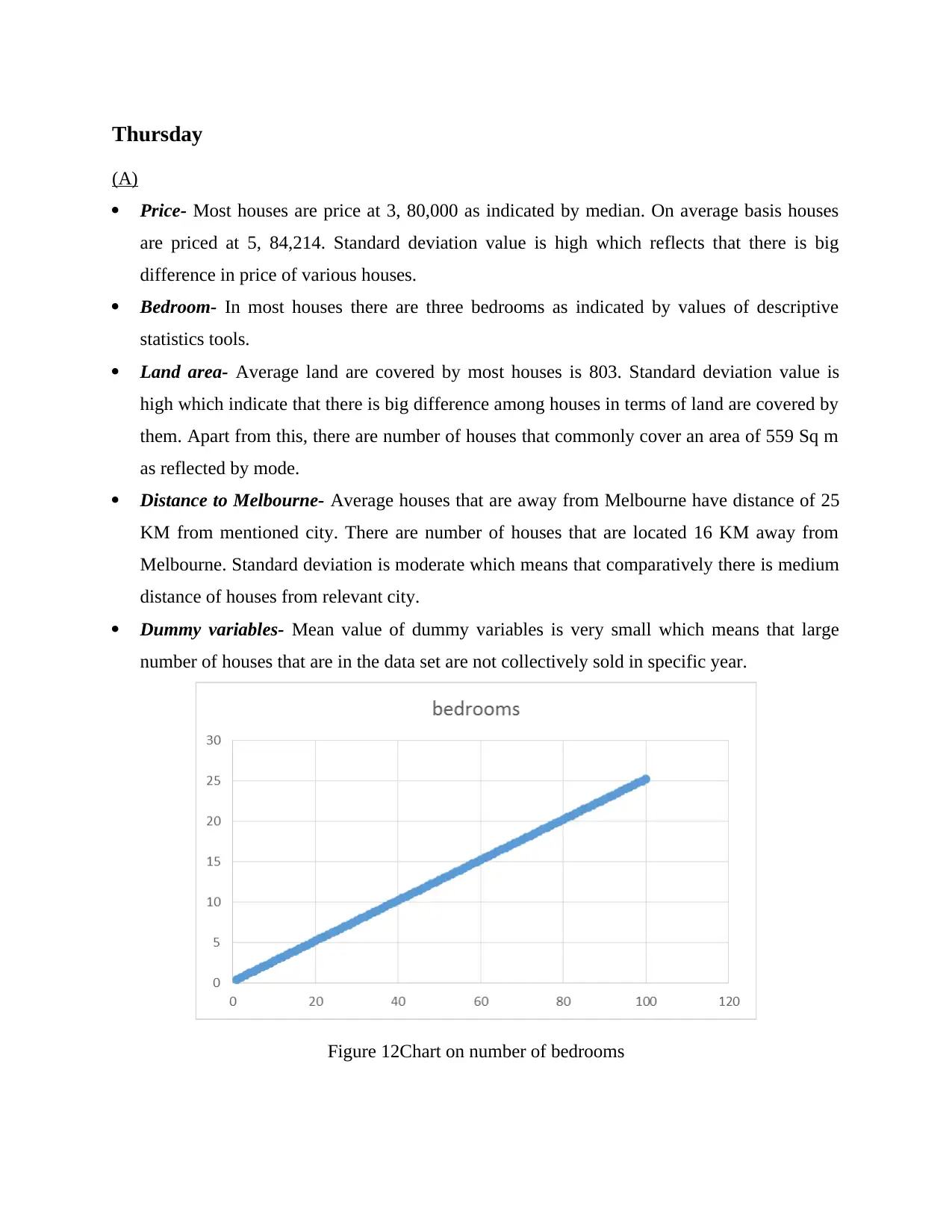
Figure 12Chart on number of bedrooms

Figure 13Chart on price of homes
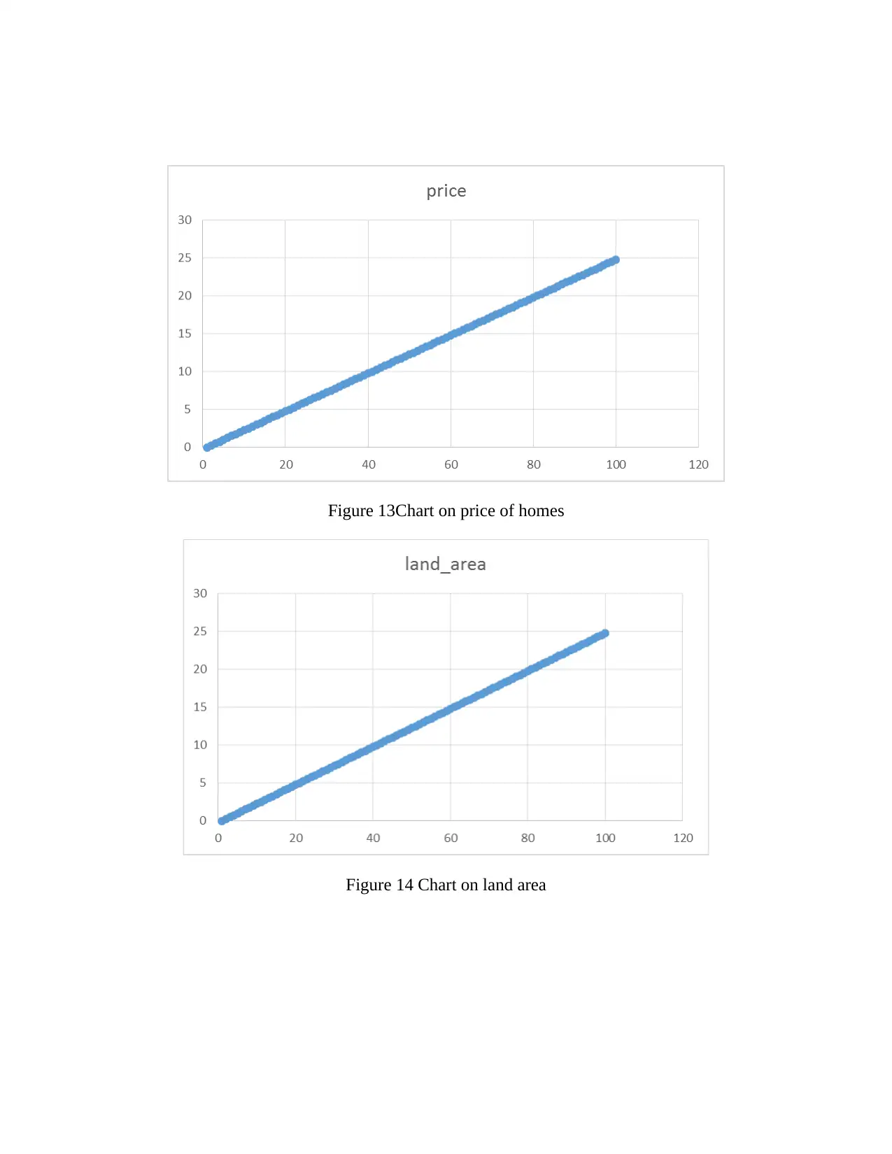
Figure 14 Chart on land area

Figure 15 Chart on mile distance
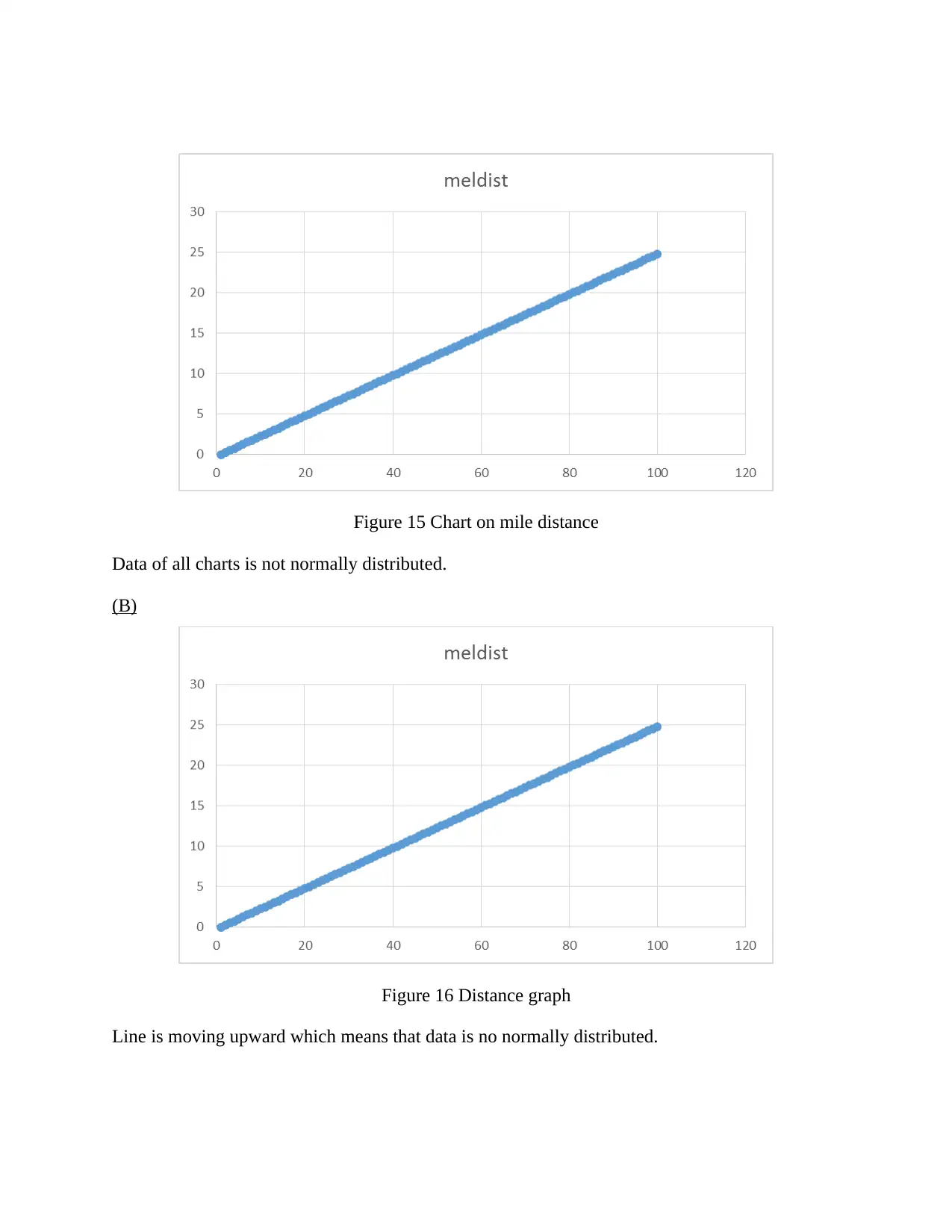
Data of all charts is not normally distributed.
(B)
Figure 16 Distance graph
Line is moving upward which means that data is no normally distributed.

©
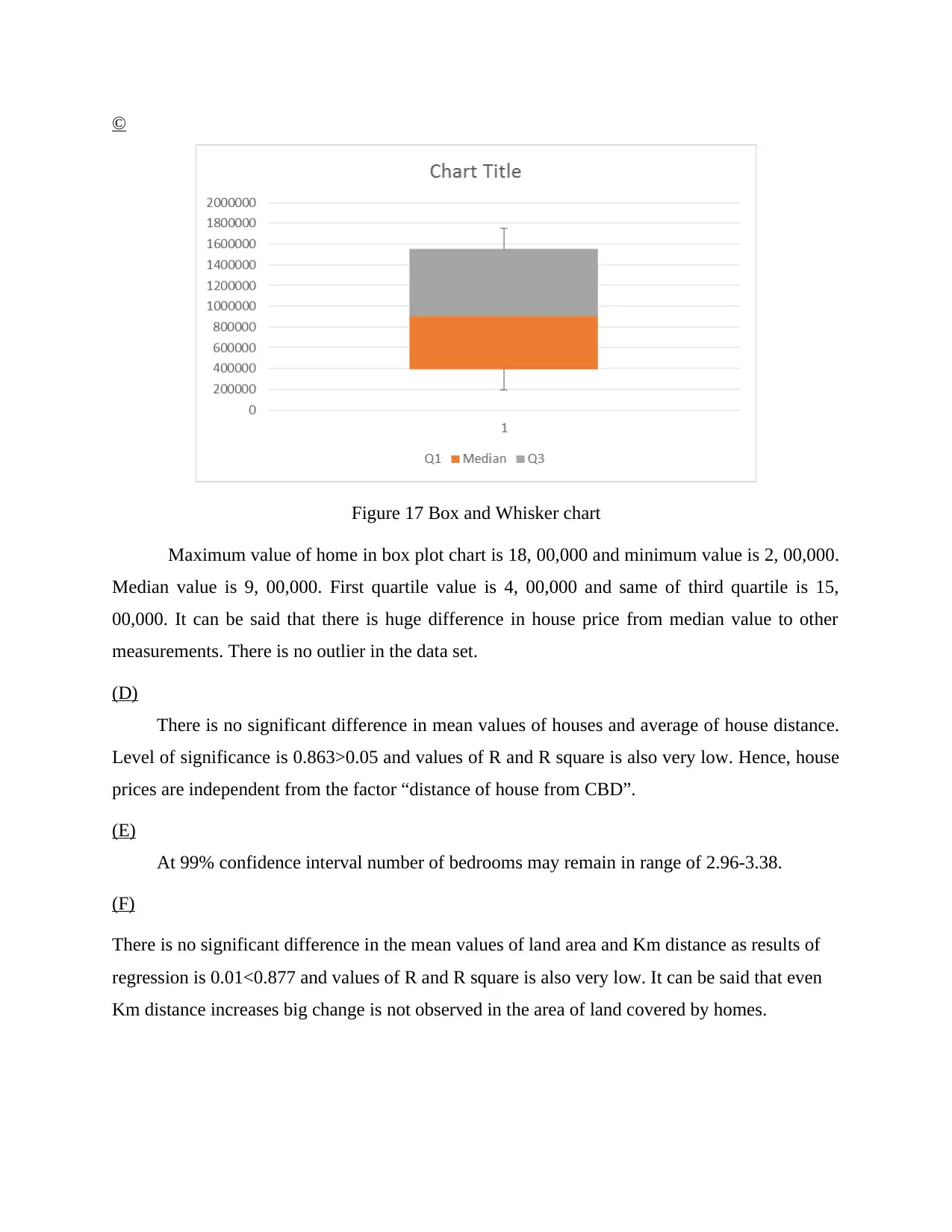
Figure 17 Box and Whisker chart
Maximum value of home in box plot chart is 18, 00,000 and minimum value is 2, 00,000.
Median value is 9, 00,000. First quartile value is 4, 00,000 and same of third quartile is 15,
00,000. It can be said that there is huge difference in house price from median value to other
measurements. There is no outlier in the data set.
(D)
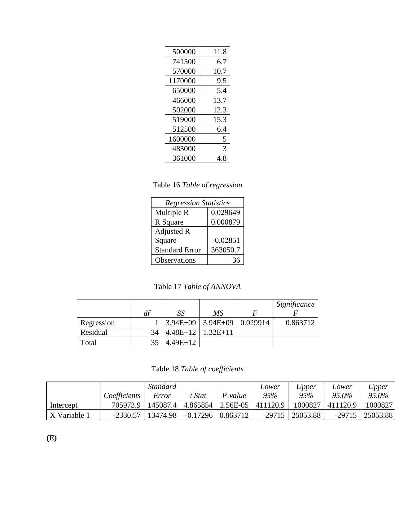
There is no significant difference in mean values of houses and average of house distance.
Level of significance is 0.863>0.05 and values of R and R square is also very low. Hence, house
prices are independent from the factor “distance of house from CBD”.
(E)
At 99% confidence interval number of bedrooms may remain in range of 2.96-3.38.
(F)
There is no significant difference in the mean values of land area and Km distance as results of
regression is 0.01<0.877 and values of R and R square is also very low. It can be said that even
Km distance increases big change is not observed in the area of land covered by homes.

(G)
There is no significant difference in mean value of price of houses and other independent
variables. This is proved from the fact that value of R and R square is 0.53 and 0.28. Apart from
this level of significance is 4.19>0.05.
(H)
Coefficient of variable distance is not statistically significant as its value if 5>0.05.
(I)
In case of bedrooms and land area value is significant as level of significance is less than
0.05. However, in case of other variables statistically different than zero. These results comes in
existence because bedroom and land area are the factors that play an important role in
determining price of house.
(J)
Value of adjusted R square is 0.23 or 23% which means that small change in independent
variables will bring mentioned percentage change in house prices. There is very small difference
in value of R and R square because addition of new variable is not bringing any change in results
produced by model.
(K)
Overall model is not statistically significant because value of P 4.19>0.005.
(L)
If in any area increasingly homes are constructed then price of mentioned property will
elevate. Hence, apart from bedrooms and land area it is another factor that determine price of
house.

(M)
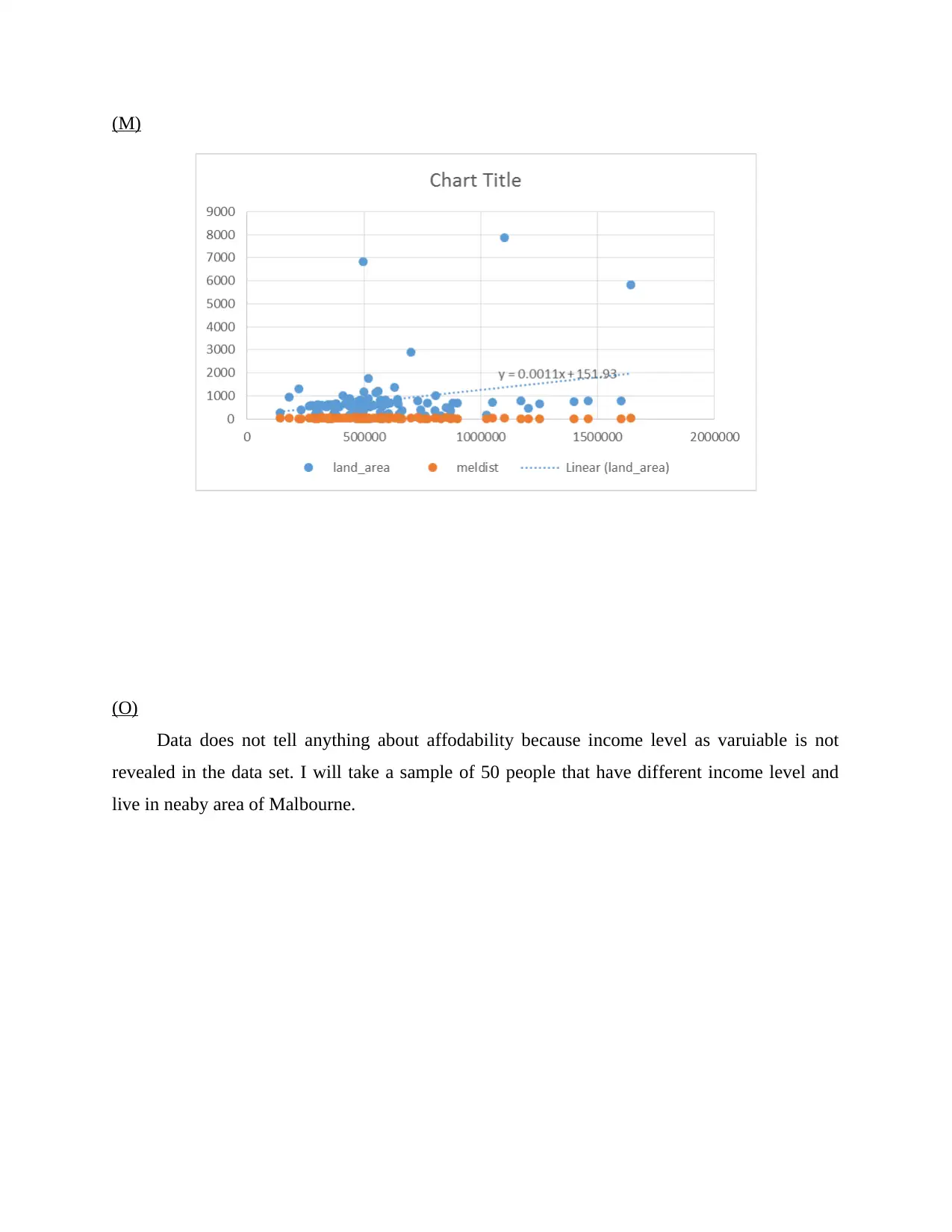
(O)
Data does not tell anything about affodability because income level as varuiable is not
revealed in the data set. I will take a sample of 50 people that have different income level and
live in neaby area of Malbourne.

Tuesday
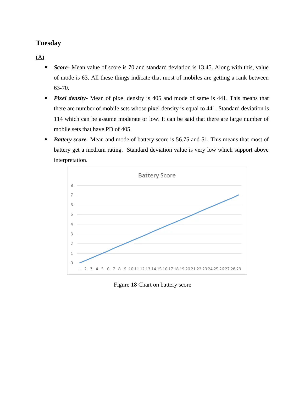
(A)
 Score- Mean value of score is 70 and standard deviation is 13.45. Along with this, value
of mode is 63. All these things indicate that most of mobiles are getting a rank between
63-70.
 Pixel density- Mean of pixel density is 405 and mode of same is 441. This means that
there are number of mobile sets whose pixel density is equal to 441. Standard deviation is
114 which can be assume moderate or low. It can be said that there are large number of
mobile sets that have PD of 405.
 Battery score- Mean and mode of battery score is 56.75 and 51. This means that most of
battery get a medium rating. Standard deviation value is very low which support above
interpretation.
Figure 18 Chart on battery score

Figure 19 Chart on pic density
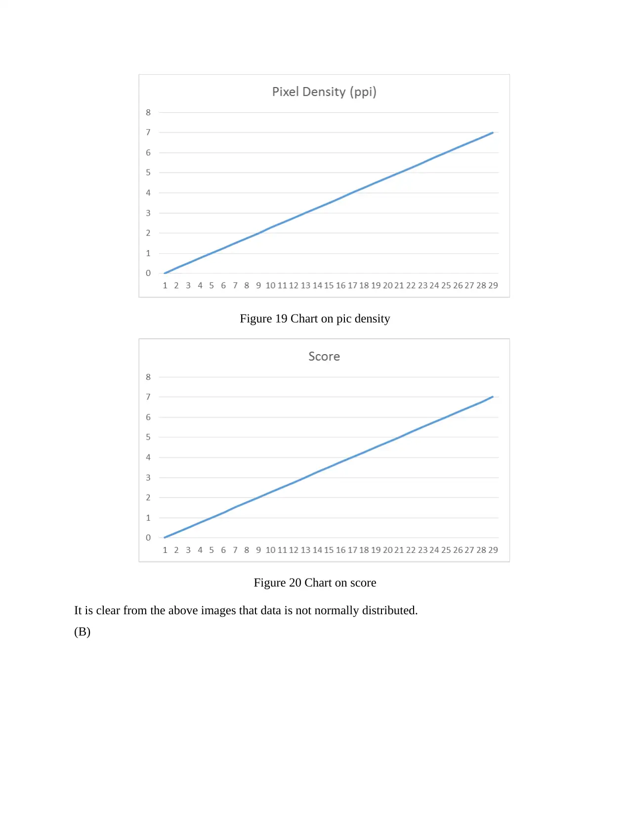
Figure 20 Chart on score
It is clear from the above images that data is not normally distributed.
(B)

Figure 21 Chart on review score
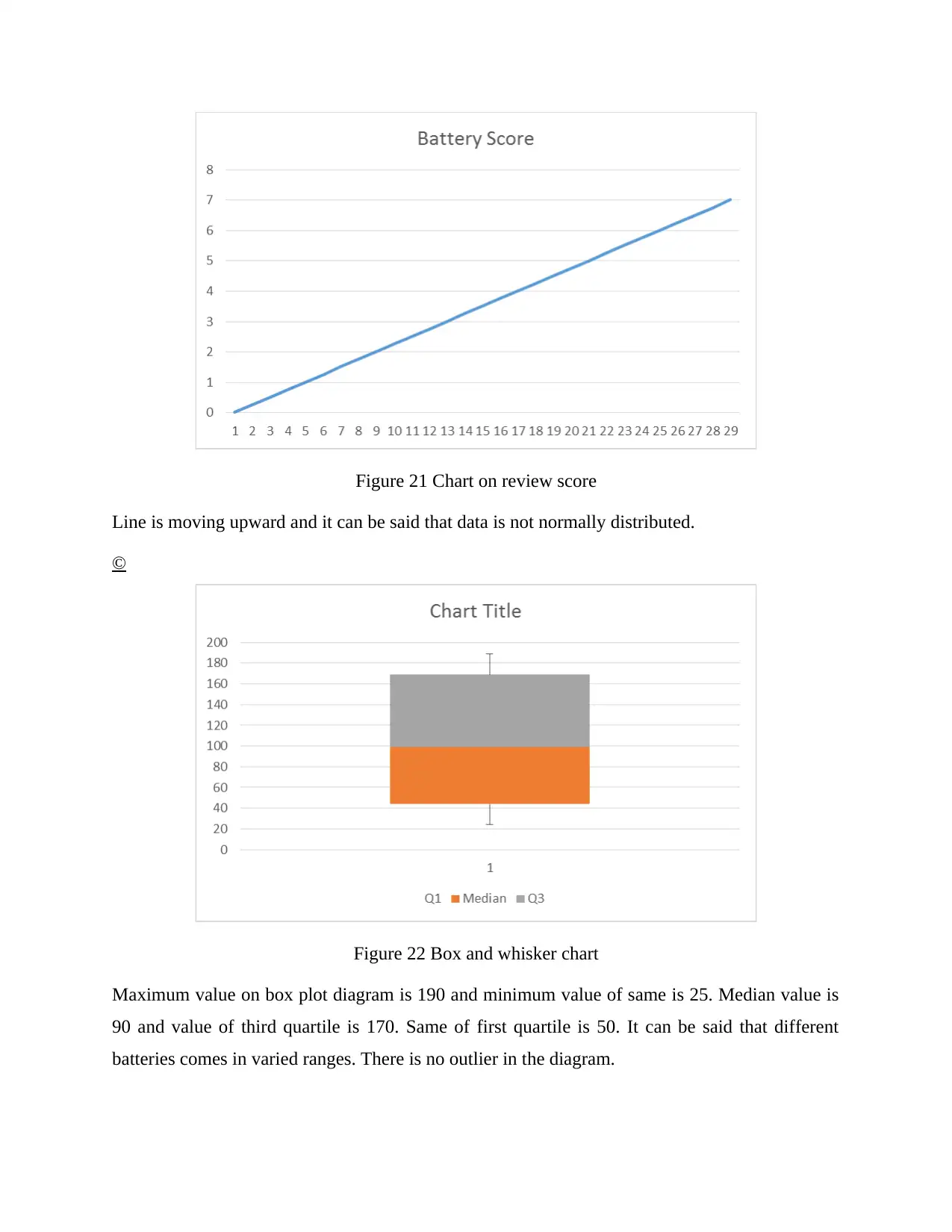
Line is moving upward and it can be said that data is not normally distributed.
©
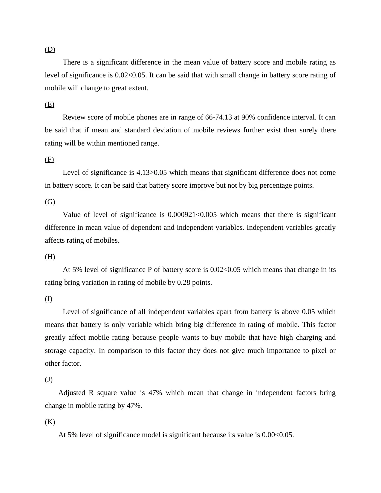
Figure 22 Box and whisker chart
Maximum value on box plot diagram is 190 and minimum value of same is 25. Median value is
90 and value of third quartile is 170. Same of first quartile is 50. It can be said that different
batteries comes in varied ranges. There is no outlier in the diagram.

(D)
There is a significant difference in the mean value of battery score and mobile rating as
level of significance is 0.02<0.05. It can be said that with small change in battery score rating of
mobile will change to great extent.
(E)
Review score of mobile phones are in range of 66-74.13 at 90% confidence interval. It can
be said that if mean and standard deviation of mobile reviews further exist then surely there
rating will be within mentioned range.
(F)
Level of significance is 4.13>0.05 which means that significant difference does not come
in battery score. It can be said that battery score improve but not by big percentage points.
(G)
Value of level of significance is 0.000921<0.005 which means that there is significant
difference in mean value of dependent and independent variables. Independent variables greatly
affects rating of mobiles.
(H)
At 5% level of significance P of battery score is 0.02<0.05 which means that change in its
rating bring variation in rating of mobile by 0.28 points.
(I)
Level of significance of all independent variables apart from battery is above 0.05 which
means that battery is only variable which bring big difference in rating of mobile. This factor
greatly affect mobile rating because people wants to buy mobile that have high charging and
storage capacity. In comparison to this factor they does not give much importance to pixel or
other factor.
(J)
Adjusted R square value is 47% which mean that change in independent factors bring
change in mobile rating by 47%.
(K)
At 5% level of significance model is significant because its value is 0.00<0.05.

(L)
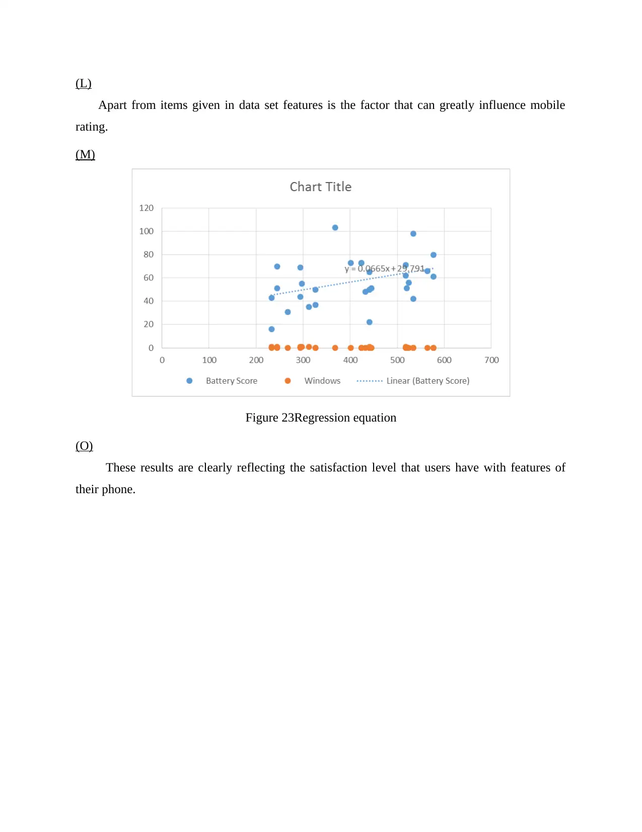
Apart from items given in data set features is the factor that can greatly influence mobile
rating.
(M)
Figure 23Regression equation
(O)
These results are clearly reflecting the satisfaction level that users have with features of
their phone.

Wednesday
(A)
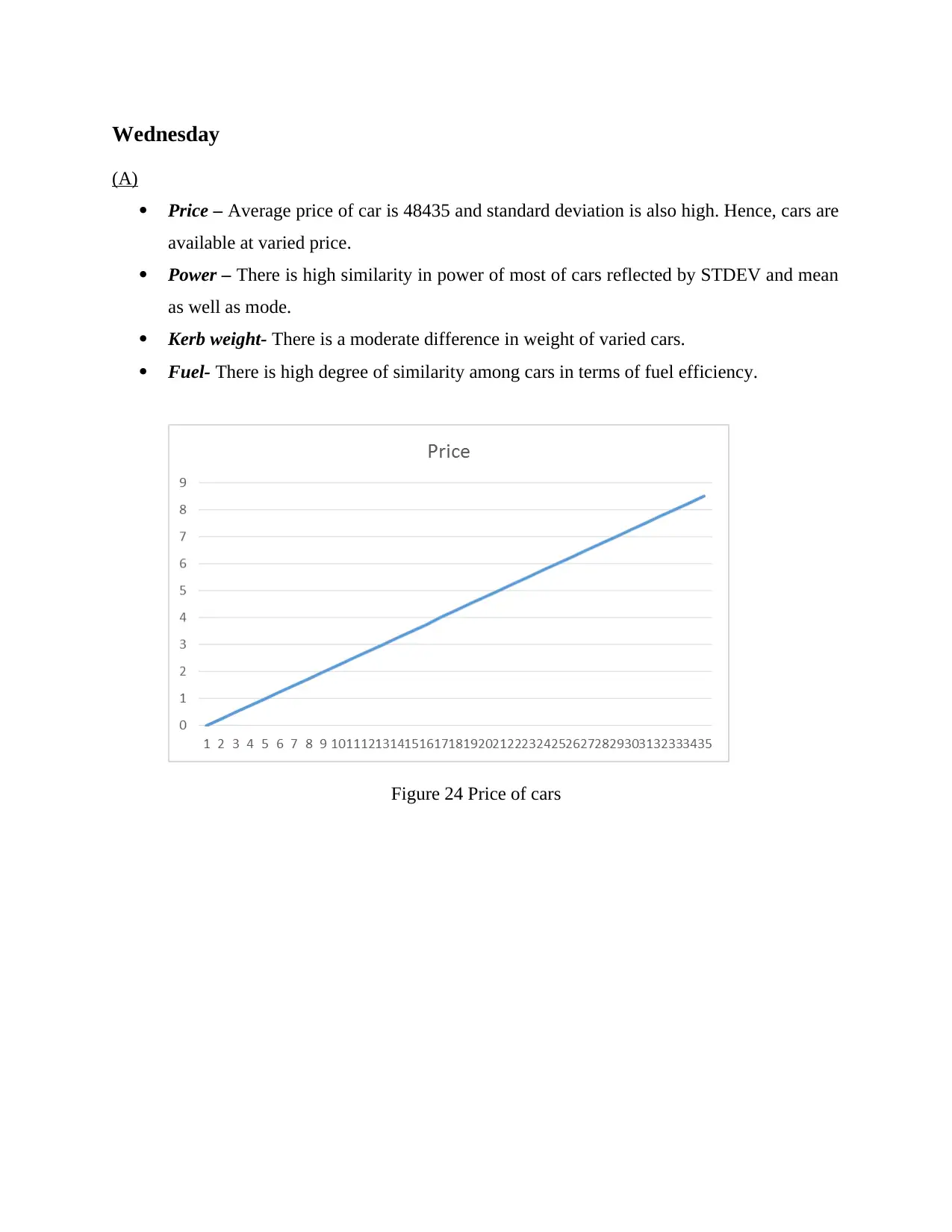
 Price – Average price of car is 48435 and standard deviation is also high. Hence, cars are
available at varied price.
 Power – There is high similarity in power of most of cars reflected by STDEV and mean
as well as mode.
 Kerb weight- There is a moderate difference in weight of varied cars.
 Fuel- There is high degree of similarity among cars in terms of fuel efficiency.
Figure 24 Price of cars

Figure 25 Power capacity of car
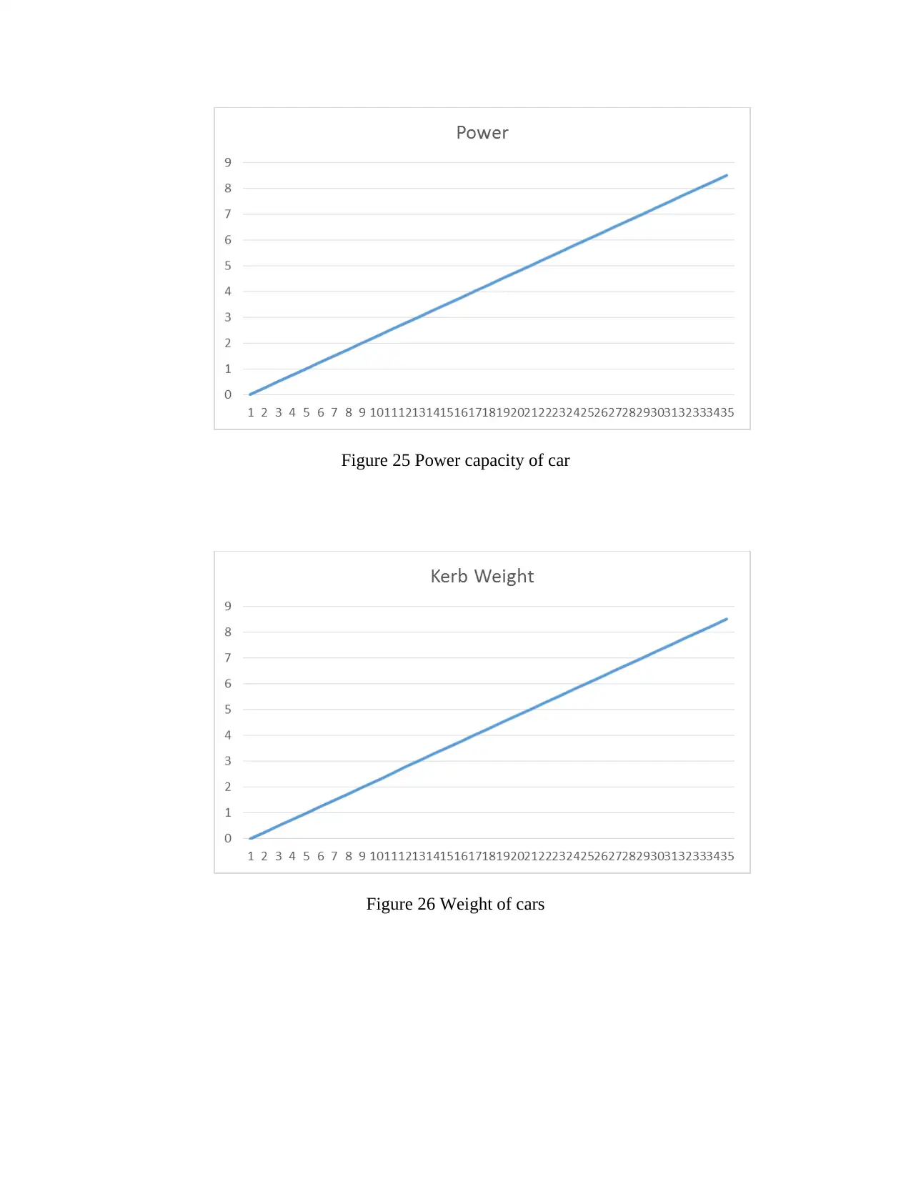
Figure 26 Weight of cars

Figure 27 Fuel efficiency of car
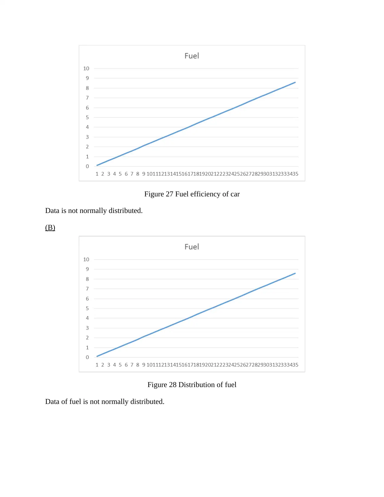
Data is not normally distributed.
(B)
Figure 28 Distribution of fuel
Data of fuel is not normally distributed.

©
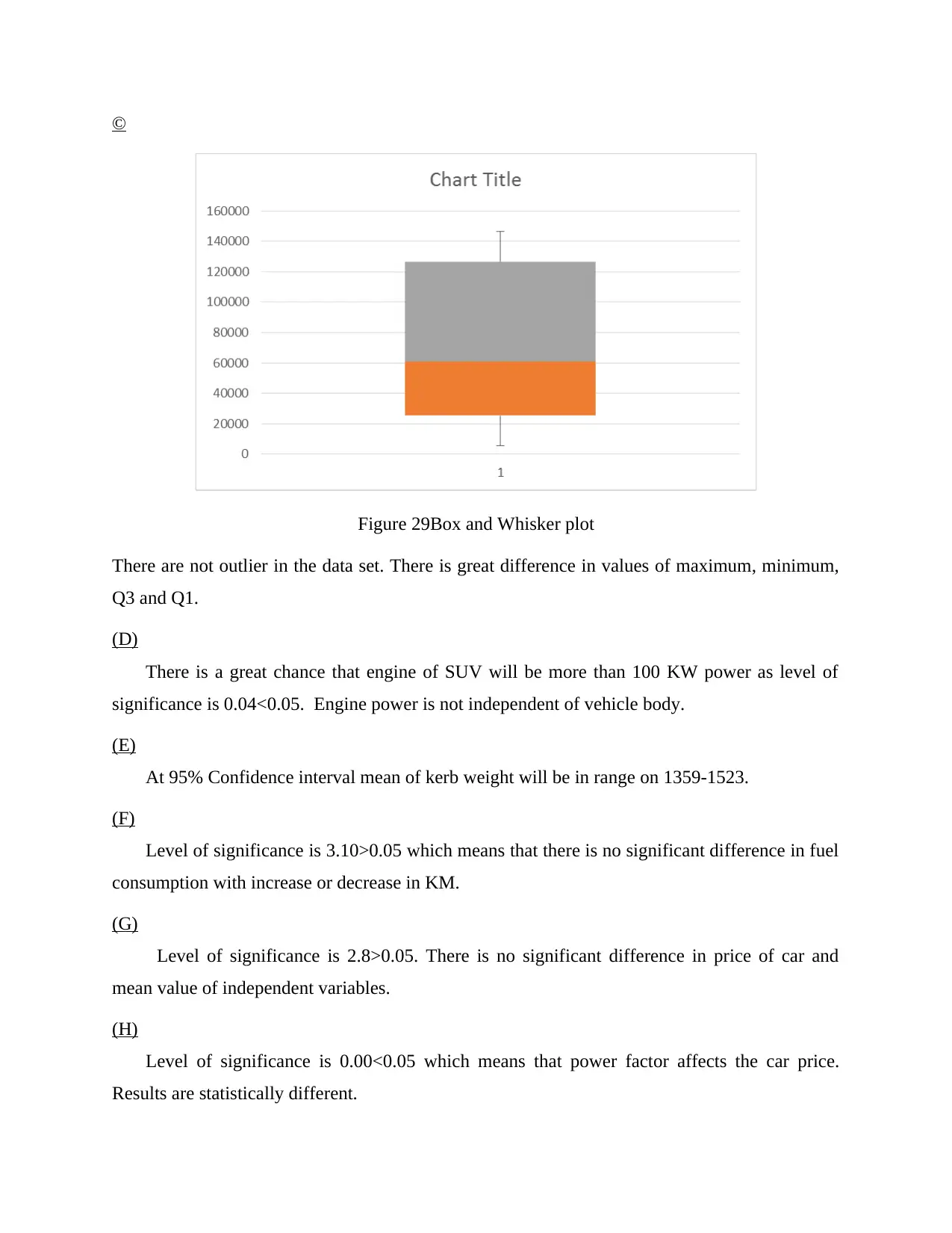
Figure 29Box and Whisker plot
There are not outlier in the data set. There is great difference in values of maximum, minimum,
Q3 and Q1.
(D)
There is a great chance that engine of SUV will be more than 100 KW power as level of
significance is 0.04<0.05. Engine power is not independent of vehicle body.
(E)
At 95% Confidence interval mean of kerb weight will be in range on 1359-1523.
(F)
Level of significance is 3.10>0.05 which means that there is no significant difference in fuel
consumption with increase or decrease in KM.
(G)
Level of significance is 2.8>0.05. There is no significant difference in price of car and
mean value of independent variables.
(H)
Level of significance is 0.00<0.05 which means that power factor affects the car price.
Results are statistically different.

(I)
Apart from power no other factor is significantly different as value of level of significance is
above 0.05 in all cases.
(J)
Value of adjusted R square is 71% which means that independent factors collectively affect
price of car.
(K)
Overall model is not significantly different as level of significance is 2.8>0.05.
(L)
Apart from factors considered in analysis demand is another factor that influence price of
cars.
(M)
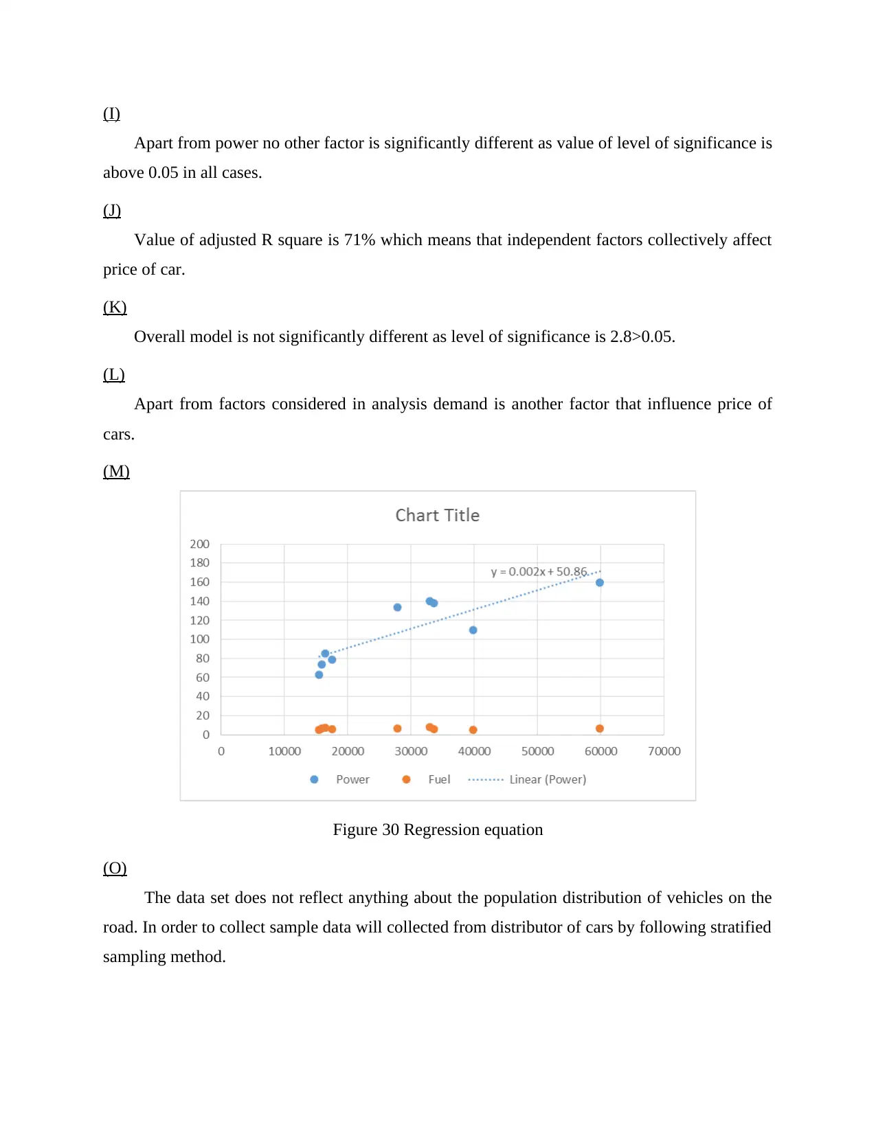
Figure 30 Regression equation
(O)
The data set does not reflect anything about the population distribution of vehicles on the
road. In order to collect sample data will collected from distributor of cars by following stratified
sampling method.

APPENDIX
(D)
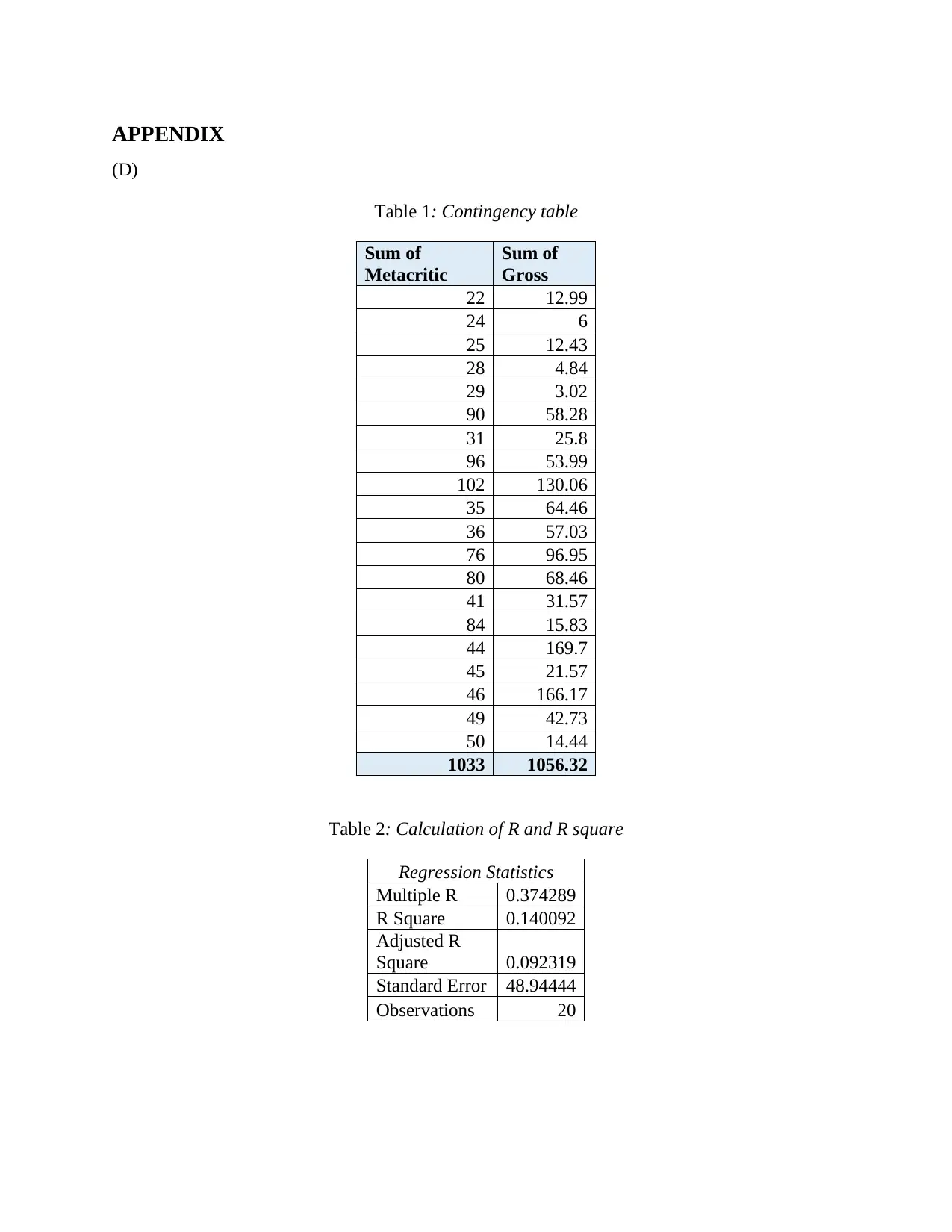
Table 1: Contingency table
Sum of
Metacritic
Sum of
Gross
22 12.99
24 6
25 12.43
28 4.84
29 3.02
90 58.28
31 25.8
96 53.99
102 130.06
35 64.46
36 57.03
76 96.95
80 68.46
41 31.57
84 15.83
44 169.7
45 21.57
46 166.17
49 42.73
50 14.44
1033 1056.32
Table 2: Calculation of R and R square
Regression Statistics
Multiple R 0.374289
R Square 0.140092
Adjusted R
Square 0.092319
Standard Error 48.94444
Observations 20

Table 3: Calculation of ANNOVA
df SS MS F
Significance
F
Regression 1 7024.901 7024.901 2.932469 0.103987736
Residual 18 43120.05 2395.558
Total 19 50144.95
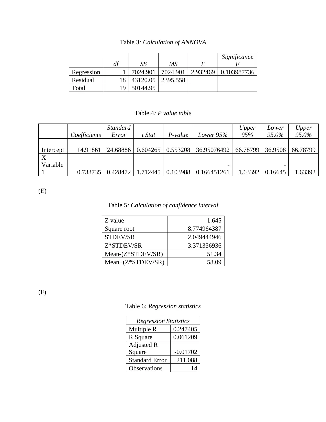
Table 4: P value table
Coefficients
Standard
Error t Stat P-value Lower 95%
Upper
95%
Lower
95.0%
Upper
95.0%
Intercept 14.91861 24.68886 0.604265 0.553208
-
36.95076492 66.78799
-
36.9508 66.78799
X
Variable
1 0.733735 0.428472 1.712445 0.103988
-
0.166451261 1.63392
-
0.16645 1.63392
(E)
Table 5: Calculation of confidence interval
Z value 1.645
Square root 8.774964387
STDEV/SR 2.049444946
Z*STDEV/SR 3.371336936
Mean-(Z*STDEV/SR) 51.34
Mean+(Z*STDEV/SR) 58.09
(F)
Table 6: Regression statistics
Regression Statistics
Multiple R 0.247405
R Square 0.061209
Adjusted R
Square -0.01702
Standard Error 211.088
Observations 14

Table 7: ANNOVA
df SS MS F
Significance
F
Regression 1 34862.36 34862.36 0.782401 0.393786
Residual 12 534698 44558.16
Total 13 569560.3
Table 8: Calculation of t-stat
Coefficients
Standard
Error t Stat P-value
Lower
95%
Upper
95%
Lower
90.0%
Upper
90.0%
Intercept 170.7429 56.41565 3.026516 0.010535 47.82371 293.662 70.19394 271.2918
X
Variable
1 0 0 65535 #NUM! 0 0 0 0
(G)
Table 9: Calculation of R and R square
Regression Statistics
Multiple R 0.767974572
R Square 0.589784943
Adjusted R Square 0.548168923
Standard Error 75.19473967
Observations 77
Table 10: Level of significance
df SS MS F Significance F
Regression 7 560926.7 80132.38 14.17206 2.97509E-11
Residual 69 390143.2 5654.249
Total 76 951069.8
(H)
Coefficient
s
Standard
Error t Stat
P-
value
Lower
95%
Upper
95%
Lower
95.0%
Upper
95.0%
Intercept
-
182.24412
96 41.92349
-
4.3470
6
4.65E-
05
-
265.87920
52
-
98.6091 -265.879
-
98.609053
96
X 0.0521668 0.010859 4.8037 8.75E- 0.0305027 0.07383 0.030503 0.0738309

Variable
1 36 99 06 34 1 38
(I)
Table 11: Slope coefficient estimates
Coefficients
Intercept -182.2441296
X Variable 1 0.052166836
X Variable 2 1.46684922
X Variable 3 84.99401238
X Variable 4 67.84665925
X Variable 5 3.113976435
X Variable 6 14.80120582
X Variable 7 18.19487877
(M)
Table 12: Prediction by using regression equation when review of movie is 30
b 0.0238
x 30
0.714
a 53.142
Forecast
price 53.856
Table 13: Predicted value of revenue on the basis of equation when movie is released on 4000
theaters
b 0.0238
x 4000
95.2
a 53.142
Forecast
price 80.427
Monday
(D)

Figure 31Contingency table
Business School Salary ATAR
Australian National University 50385 82
Charles Sturt University 55136 65
Curtin University 42062 70
Macquarie University 40692 80
Monash University 43928 82
Murdoch University 42078 70
Queensland University of
Technology 43006 62
RMIT University 41897 70
University of Adelaide 42946 80
University of Canberra 47485 68
University of Melbourne 57296 95
University of New England 55778 73
University of New South Wales 49665 96
University of Notre Dame Australia 43728 70
University of Queensland 43860 81
University of South Australia 42939 65
University of Sydney 52414 95
University of Tasmania 44345 65
University of Technology, Sydney 41782 69
University of Western Australia 49003 80
University of Wollongong 46703 70
Victoria University 36321 50
Western Sydney University 40806 65
Figure 32 Regression table
Regression Statistics
Multiple R 0.556412
R Square 0.309594
Adjusted R
Square 0.276718
Standard Error 9.657592
Observations 23
Figure 33 ANNOVA table
df SS MS F
Significance
F

Regression 1 878.3057 878.3057 9.416901 0.005828
Residual 21 1958.651 93.26909
Total 22 2836.957
Figure 34 Coefficient table
Coefficients
Standard
Error t Stat P-value
Lower
95%
Upper
95%
Lower
95.0%
Upper
95.0%
Intercept 20.77617 17.4747 1.188928 0.247739 -15.5645 57.1168 -15.5645 57.1168
X
Variable
1 0.001162 0.000379 3.068697 0.005828 0.000375 0.00195 0.000375 0.00195
€
Figure 35 95% Confidence interval
Z value 1.645
Square root 6.244998
STDEV/SR 889.6359
Z*STDEV/SR 1463.451
Mean-(z*stdev/sr) 42308.98
Mean+(Z*STDEV/SR) 46180
(F)
(G)
Figure 36 Statistics of regression
Regression Statistics
Multiple R 0.632738
R Square 0.400357
Adjusted R
Square 0.214261
Standard Error 4924.744
Observations 39

Figure 37ANNOVA table
df SS MS F
Significance
F
Regression 9 4.7E+08 52176895 2.151349 0.057246
Residual 29 7.03E+08 24253102
Total 38 1.17E+09
Figure 38 Table of coefficients
Coefficients
Standard
Error t Stat P-value
Lower
95%
Upper
95%
Lower
95.0%
Upper
95.0%
Intercept 14813.6 18051.82 0.820615 0.41856 -22106.5 51733.71 -22106.5 51733.71
X
Variable
1 195.0207 205.6479 0.948323 0.350801 -225.577 615.6179 -225.577 615.6179
X
Variable
2 290.0331 101.9312 2.84538 0.008057 81.56031 498.5058 81.56031 498.5058
X
Variable
3 -1765.05 3238.397 -0.54504 0.589895 -8388.31 4858.215 -8388.31 4858.215
X
Variable
4 -2802.5 2570.932 -1.09007 0.284657 -8060.65 2455.646 -8060.65 2455.646
X
Variable
5 -5432.1 2931.041 -1.8533 0.074039 -11426.8 562.5505 -11426.8 562.5505
X
Variable
6 -3443.48 3261.057 -1.05594 0.299713 -10113.1 3226.128 -10113.1 3226.128
X
Variable
7 -6109.69 4648.842 -1.31424 0.199066 -15617.6 3398.256 -15617.6 3398.256
X
Variable
8 -6536.68 3262.197 -2.00377 0.054516 -13208.6 135.2589 -13208.6 135.2589
X
Variable
9 -5622.26 3454.117 -1.6277 0.114407 -12686.7 1442.202 -12686.7 1442.202
(M)
b 0.0238
x 75

1.785
a 53.142
26.8877

Thursday
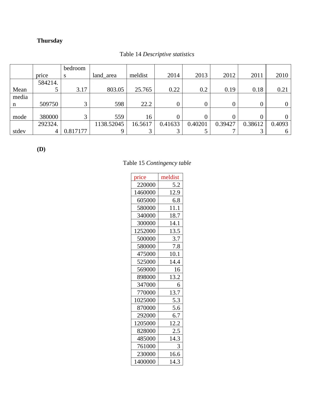
Table 14 Descriptive statistics
price
bedroom
s land_area meldist 2014 2013 2012 2011 2010
Mean
584214.
5 3.17 803.05 25.765 0.22 0.2 0.19 0.18 0.21
media
n 509750 3 598 22.2 0 0 0 0 0
mode 380000 3 559 16 0 0 0 0 0
stdev
292324.
4 0.817177
1138.52045
9
16.5617
3
0.41633
3
0.40201
5
0.39427
7
0.38612
3
0.4093
6
(D)
Table 15 Contingency table
price meldist
220000 5.2
1460000 12.9
605000 6.8
580000 11.1
340000 18.7
300000 14.1
1252000 13.5
500000 3.7
580000 7.8
475000 10.1
525000 14.4
569000 16
898000 13.2
347000 6
770000 13.7
1025000 5.3
870000 5.6
292000 6.7
1205000 12.2
828000 2.5
485000 14.3
761000 3
230000 16.6
1400000 14.3

500000 11.8
741500 6.7
570000 10.7
1170000 9.5
650000 5.4
466000 13.7
502000 12.3
519000 15.3
512500 6.4
1600000 5
485000 3
361000 4.8
Table 16 Table of regression
Regression Statistics
Multiple R 0.029649
R Square 0.000879
Adjusted R
Square -0.02851
Standard Error 363050.7
Observations 36
Table 17 Table of ANNOVA
df SS MS F
Significance
F
Regression 1 3.94E+09 3.94E+09 0.029914 0.863712
Residual 34 4.48E+12 1.32E+11
Total 35 4.49E+12
Table 18 Table of coefficients
Coefficients
Standard
Error t Stat P-value
Lower
95%
Upper
95%
Lower
95.0%
Upper
95.0%
Intercept 705973.9 145087.4 4.865854 2.56E-05 411120.9 1000827 411120.9 1000827
X Variable 1 -2330.57 13474.98 -0.17296 0.863712 -29715 25053.88 -29715 25053.88
(E)

Table 19 Range of bedrooms at 99% confidence interval
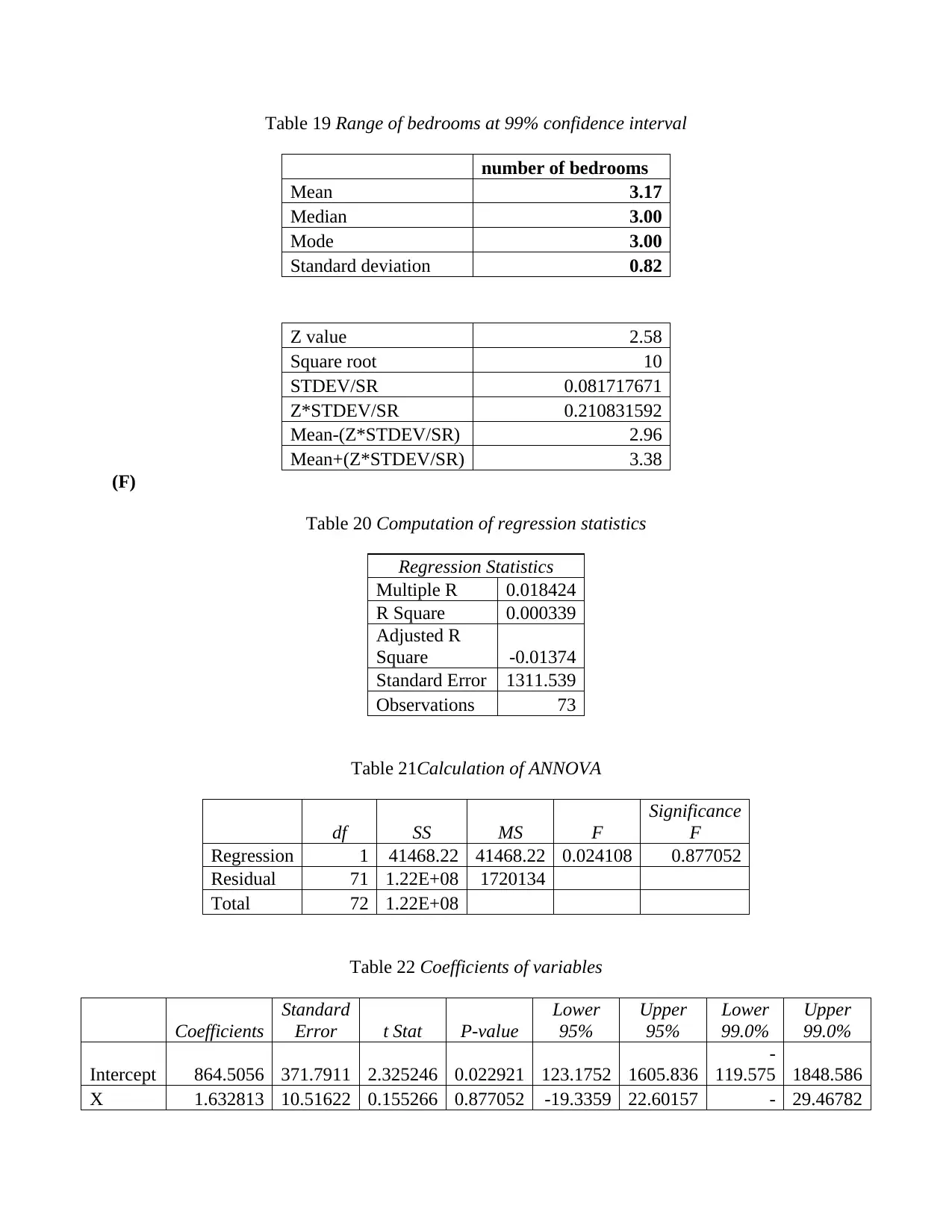
number of bedrooms
Mean 3.17
Median 3.00
Mode 3.00
Standard deviation 0.82
Z value 2.58
Square root 10
STDEV/SR 0.081717671
Z*STDEV/SR 0.210831592
Mean-(Z*STDEV/SR) 2.96
Mean+(Z*STDEV/SR) 3.38
(F)
Table 20 Computation of regression statistics
Regression Statistics
Multiple R 0.018424
R Square 0.000339
Adjusted R
Square -0.01374
Standard Error 1311.539
Observations 73
Table 21Calculation of ANNOVA
df SS MS F
Significance
F
Regression 1 41468.22 41468.22 0.024108 0.877052
Residual 71 1.22E+08 1720134
Total 72 1.22E+08
Table 22 Coefficients of variables
Coefficients
Standard
Error t Stat P-value
Lower
95%
Upper
95%
Lower
99.0%
Upper
99.0%
Intercept 864.5056 371.7911 2.325246 0.022921 123.1752 1605.836
-
119.575 1848.586
X 1.632813 10.51622 0.155266 0.877052 -19.3359 22.60157 - 29.46782

Variable
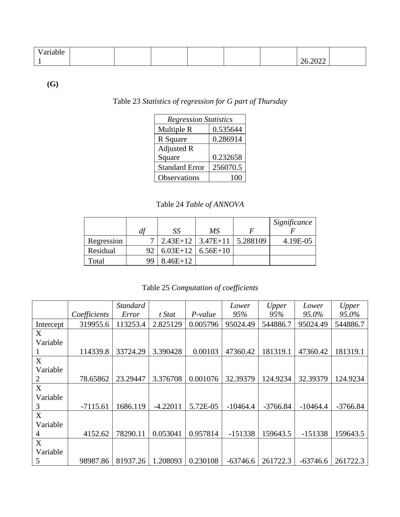
1 26.2022
(G)
Table 23 Statistics of regression for G part of Thursday
Regression Statistics
Multiple R 0.535644
R Square 0.286914
Adjusted R
Square 0.232658
Standard Error 256070.5
Observations 100
Table 24 Table of ANNOVA
df SS MS F
Significance
F
Regression 7 2.43E+12 3.47E+11 5.288109 4.19E-05
Residual 92 6.03E+12 6.56E+10
Total 99 8.46E+12
Table 25 Computation of coefficients
Coefficients
Standard
Error t Stat P-value
Lower
95%
Upper
95%
Lower
95.0%
Upper
95.0%
Intercept 319955.6 113253.4 2.825129 0.005796 95024.49 544886.7 95024.49 544886.7
X
Variable
1 114339.8 33724.29 3.390428 0.00103 47360.42 181319.1 47360.42 181319.1
X
Variable
2 78.65862 23.29447 3.376708 0.001076 32.39379 124.9234 32.39379 124.9234
X
Variable
3 -7115.61 1686.119 -4.22011 5.72E-05 -10464.4 -3766.84 -10464.4 -3766.84
X
Variable
4 4152.62 78290.11 0.053041 0.957814 -151338 159643.5 -151338 159643.5
X
Variable
5 98987.86 81937.26 1.208093 0.230108 -63746.6 261722.3 -63746.6 261722.3

X
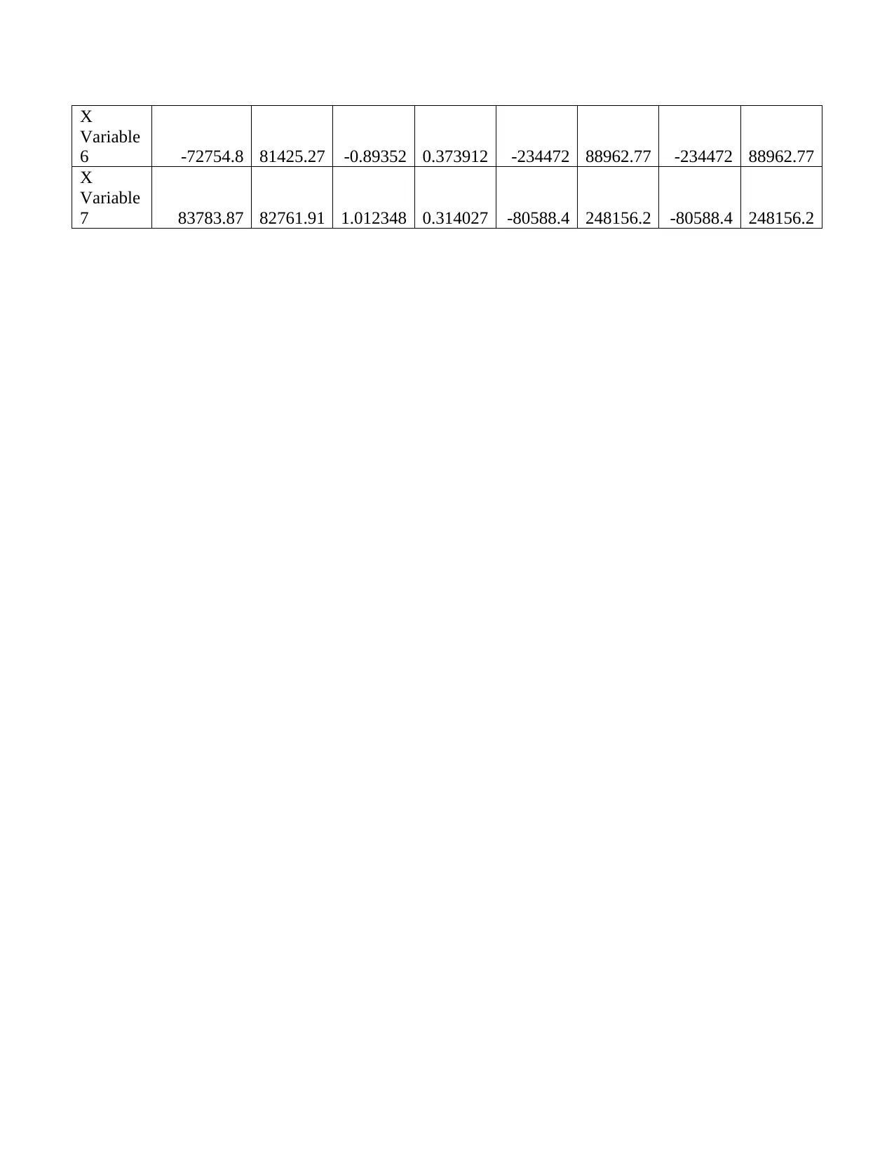
Variable
6 -72754.8 81425.27 -0.89352 0.373912 -234472 88962.77 -234472 88962.77
X
Variable
7 83783.87 82761.91 1.012348 0.314027 -80588.4 248156.2 -80588.4 248156.2

Tuesday
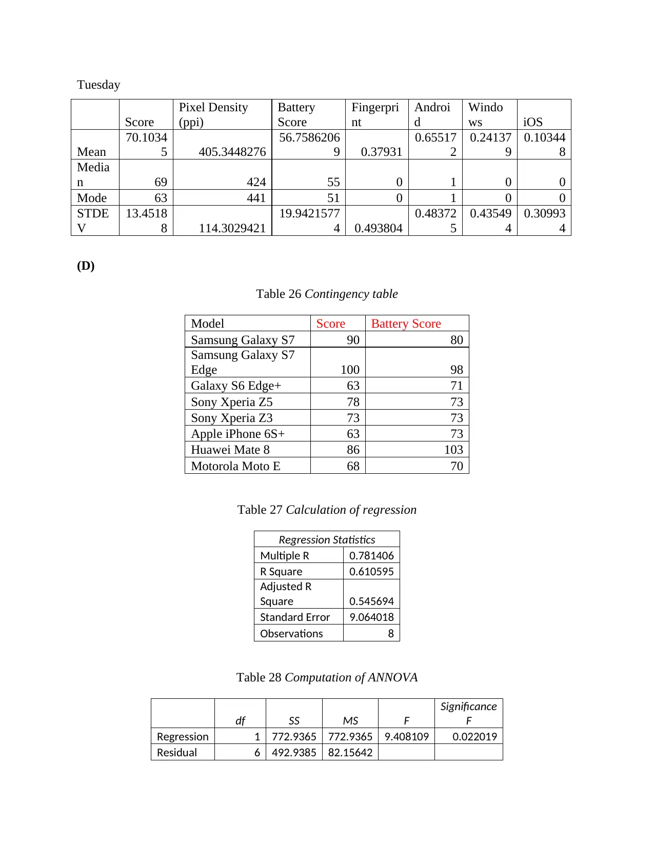
Score
Pixel Density
(ppi)
Battery
Score
Fingerpri
nt
Androi
d
Windo
ws iOS
Mean
70.1034
5 405.3448276
56.7586206
9 0.37931
0.65517
2
0.24137
9
0.10344
8
Media
n 69 424 55 0 1 0 0
Mode 63 441 51 0 1 0 0
STDE
V
13.4518
8 114.3029421
19.9421577
4 0.493804
0.48372
5
0.43549
4
0.30993
4
(D)
Table 26 Contingency table
Model Score Battery Score
Samsung Galaxy S7 90 80
Samsung Galaxy S7
Edge 100 98
Galaxy S6 Edge+ 63 71
Sony Xperia Z5 78 73
Sony Xperia Z3 73 73
Apple iPhone 6S+ 63 73
Huawei Mate 8 86 103
Motorola Moto E 68 70
Table 27 Calculation of regression
Regression Statistics
Multiple R 0.781406
R Square 0.610595
Adjusted R
Square 0.545694
Standard Error 9.064018
Observations 8
Table 28 Computation of ANNOVA
df SS MS F
Significance
F
Regression 1 772.9365 772.9365 9.408109 0.022019
Residual 6 492.9385 82.15642

Total 7 1265.875
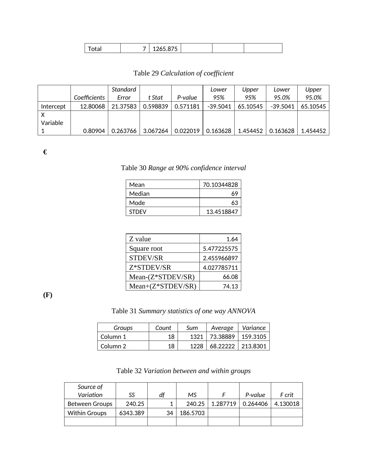
Table 29 Calculation of coefficient
Coefficients
Standard
Error t Stat P-value
Lower
95%
Upper
95%
Lower
95.0%
Upper
95.0%
Intercept 12.80068 21.37583 0.598839 0.571181 -39.5041 65.10545 -39.5041 65.10545
X
Variable
1 0.80904 0.263766 3.067264 0.022019 0.163628 1.454452 0.163628 1.454452
€
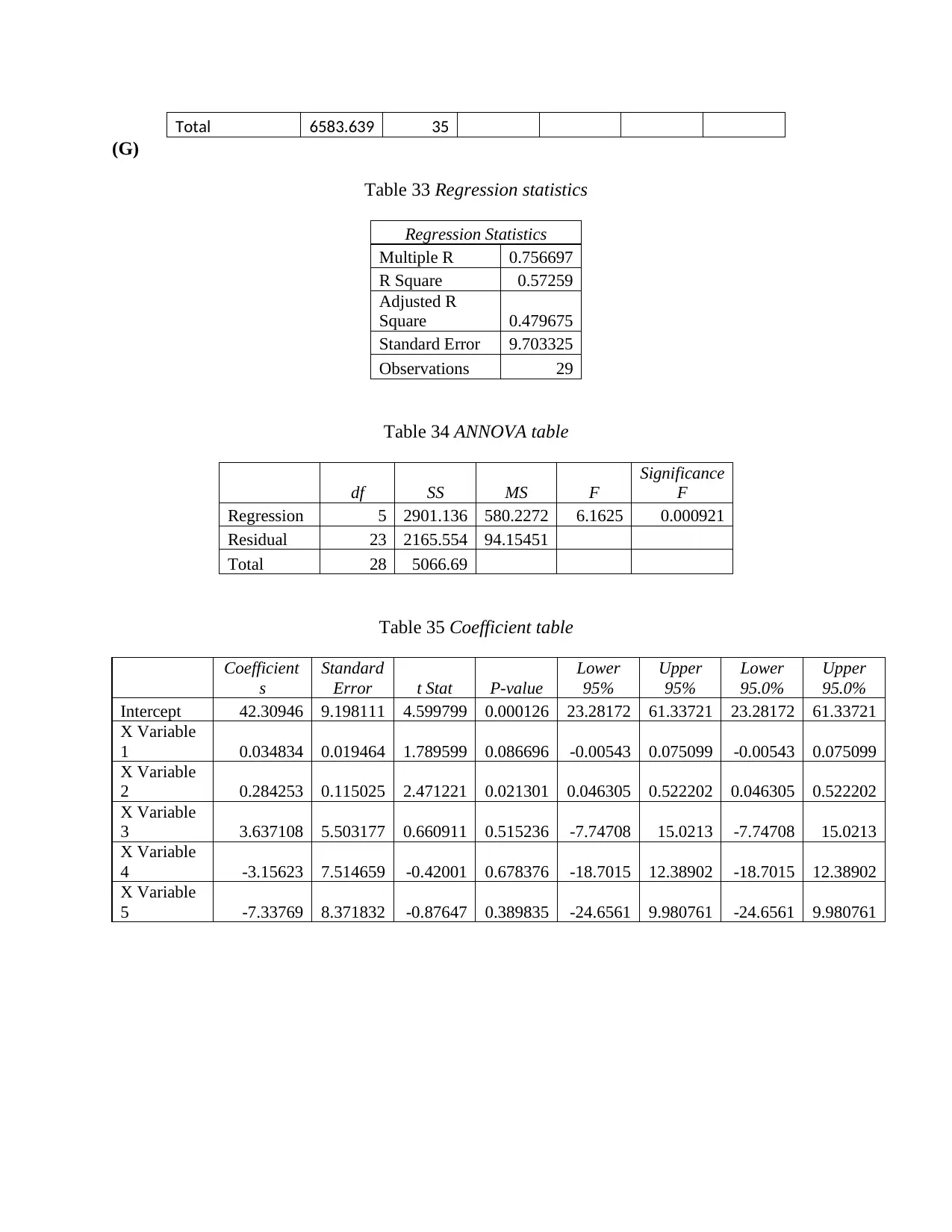
Table 30 Range at 90% confidence interval
Mean 70.10344828
Median 69
Mode 63
STDEV 13.4518847
Z value 1.64
Square root 5.477225575
STDEV/SR 2.455966897
Z*STDEV/SR 4.027785711
Mean-(Z*STDEV/SR) 66.08
Mean+(Z*STDEV/SR) 74.13
(F)
Table 31 Summary statistics of one way ANNOVA
Groups Count Sum Average Variance
Column 1 18 1321 73.38889 159.3105
Column 2 18 1228 68.22222 213.8301
Table 32 Variation between and within groups
Source of
Variation SS df MS F P-value F crit
Between Groups 240.25 1 240.25 1.287719 0.264406 4.130018
Within Groups 6343.389 34 186.5703

Total 6583.639 35
(G)
Table 33 Regression statistics
Regression Statistics
Multiple R 0.756697
R Square 0.57259
Adjusted R
Square 0.479675
Standard Error 9.703325
Observations 29
Table 34 ANNOVA table
df SS MS F
Significance
F
Regression 5 2901.136 580.2272 6.1625 0.000921
Residual 23 2165.554 94.15451
Total 28 5066.69
Table 35 Coefficient table
Coefficient
s
Standard
Error t Stat P-value
Lower
95%
Upper
95%
Lower
95.0%
Upper
95.0%
Intercept 42.30946 9.198111 4.599799 0.000126 23.28172 61.33721 23.28172 61.33721
X Variable
1 0.034834 0.019464 1.789599 0.086696 -0.00543 0.075099 -0.00543 0.075099
X Variable
2 0.284253 0.115025 2.471221 0.021301 0.046305 0.522202 0.046305 0.522202
X Variable
3 3.637108 5.503177 0.660911 0.515236 -7.74708 15.0213 -7.74708 15.0213
X Variable
4 -3.15623 7.514659 -0.42001 0.678376 -18.7015 12.38902 -18.7015 12.38902
X Variable
5 -7.33769 8.371832 -0.87647 0.389835 -24.6561 9.980761 -24.6561 9.980761

Wednesday
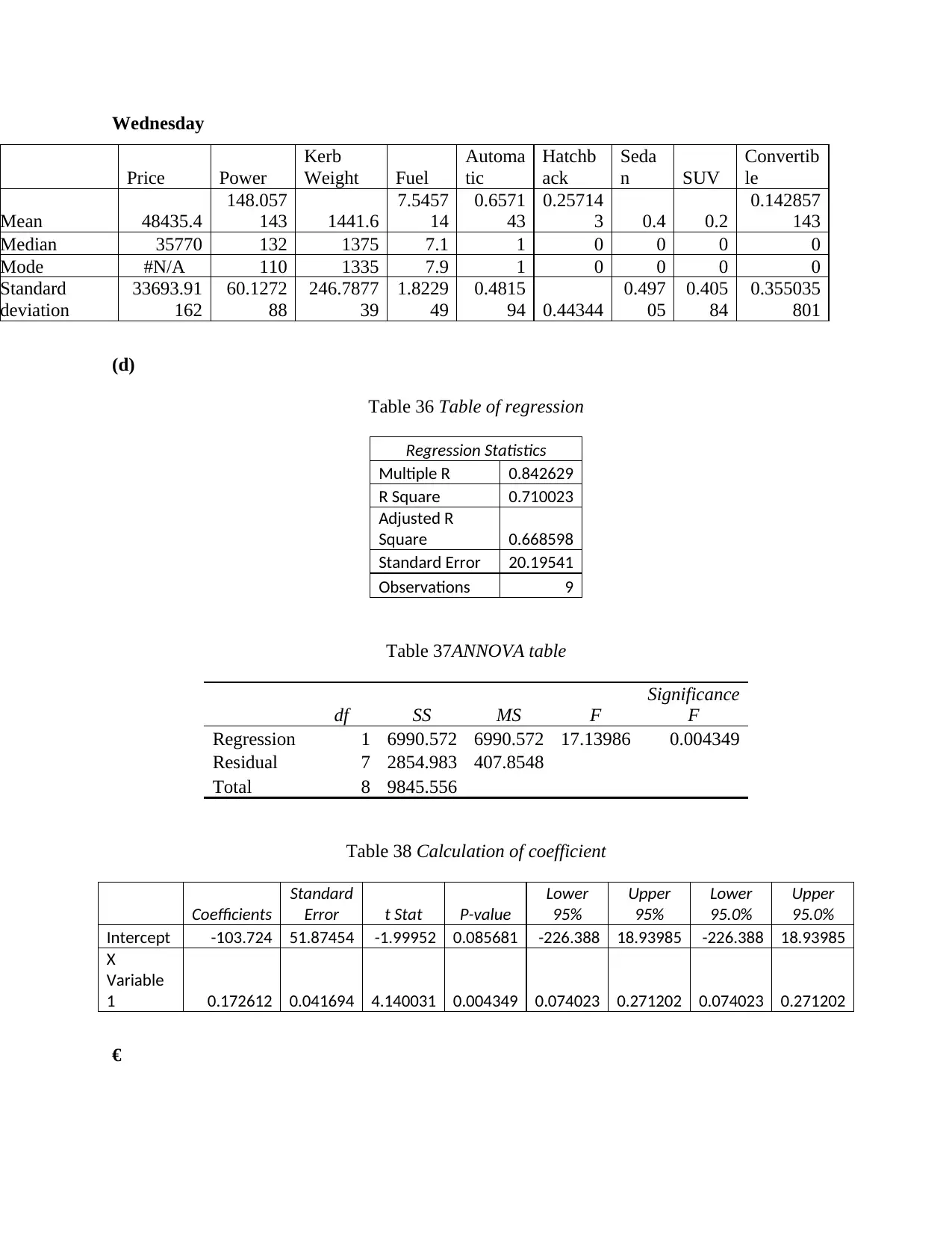
Price Power
Kerb
Weight Fuel
Automa
tic
Hatchb
ack
Seda
n SUV
Convertib
le
Mean 48435.4
148.057
143 1441.6
7.5457
14
0.6571
43
0.25714
3 0.4 0.2
0.142857
143
Median 35770 132 1375 7.1 1 0 0 0 0
Mode #N/A 110 1335 7.9 1 0 0 0 0
Standard
deviation
33693.91
162
60.1272
88
246.7877
39
1.8229
49
0.4815
94 0.44344
0.497
05
0.405
84
0.355035
801
(d)
Table 36 Table of regression
Regression Statistics
Multiple R 0.842629
R Square 0.710023
Adjusted R
Square 0.668598
Standard Error 20.19541
Observations 9
Table 37ANNOVA table
df SS MS F
Significance
F
Regression 1 6990.572 6990.572 17.13986 0.004349
Residual 7 2854.983 407.8548
Total 8 9845.556
Table 38 Calculation of coefficient
Coefficients
Standard
Error t Stat P-value
Lower
95%
Upper
95%
Lower
95.0%
Upper
95.0%
Intercept -103.724 51.87454 -1.99952 0.085681 -226.388 18.93985 -226.388 18.93985
X
Variable
1 0.172612 0.041694 4.140031 0.004349 0.074023 0.271202 0.074023 0.271202
€

Table 39 95% Confidence interval
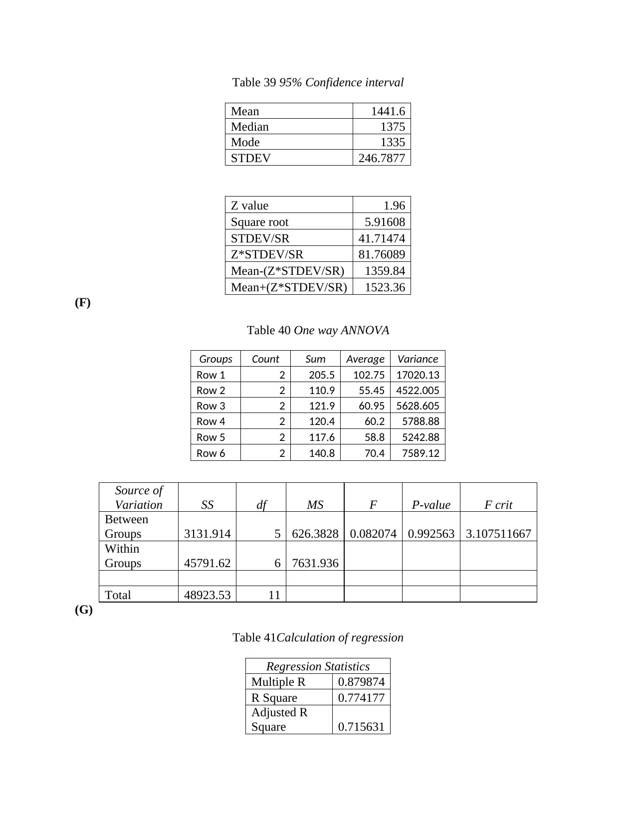
Mean 1441.6
Median 1375
Mode 1335
STDEV 246.7877
Z value 1.96
Square root 5.91608
STDEV/SR 41.71474
Z*STDEV/SR 81.76089
Mean-(Z*STDEV/SR) 1359.84
Mean+(Z*STDEV/SR) 1523.36
(F)
Table 40 One way ANNOVA
Groups Count Sum Average Variance
Row 1 2 205.5 102.75 17020.13
Row 2 2 110.9 55.45 4522.005
Row 3 2 121.9 60.95 5628.605
Row 4 2 120.4 60.2 5788.88
Row 5 2 117.6 58.8 5242.88
Row 6 2 140.8 70.4 7589.12
Source of
Variation SS df MS F P-value F crit
Between
Groups 3131.914 5 626.3828 0.082074 0.992563 3.107511667
Within
Groups 45791.62 6 7631.936
Total 48923.53 11
(G)
Table 41Calculation of regression
Regression Statistics
Multiple R 0.879874
R Square 0.774177
Adjusted R
Square 0.715631

Standard Error 17967.71
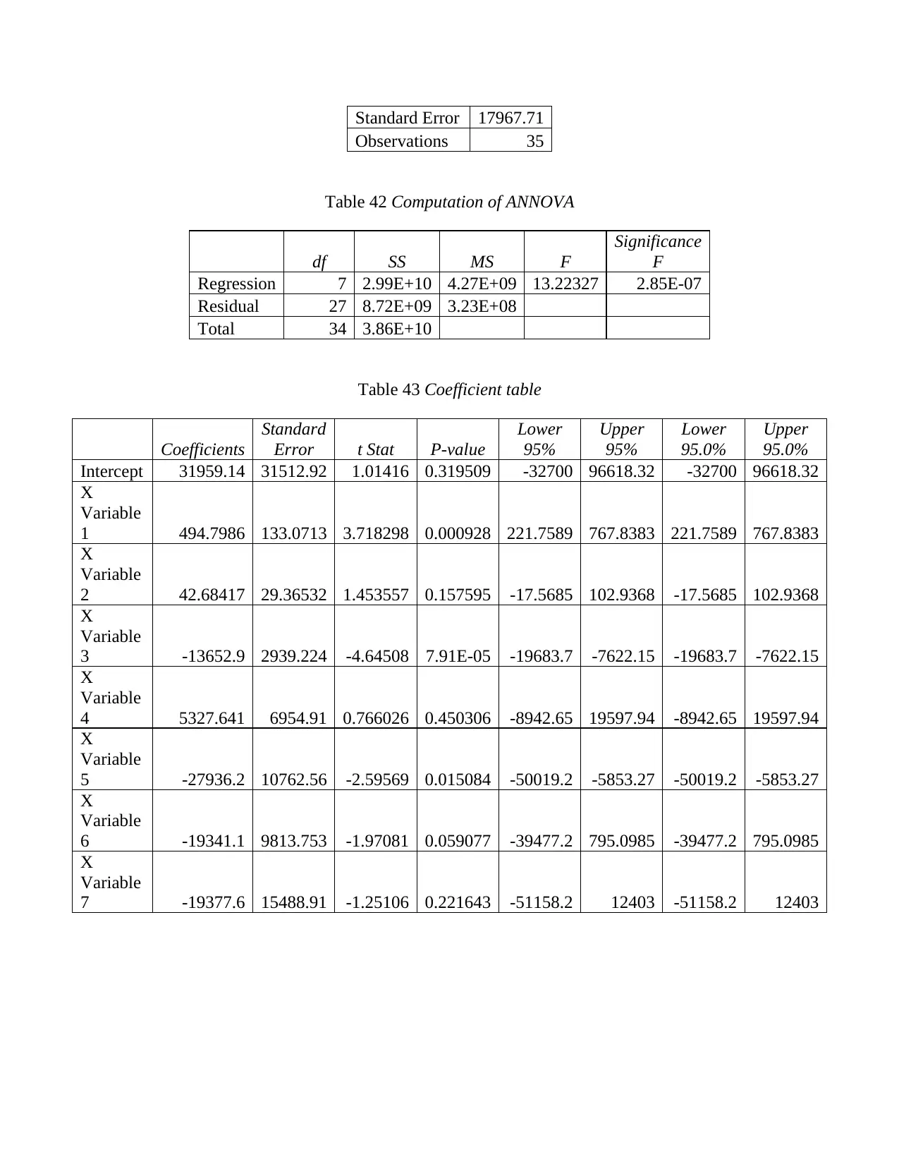
Observations 35
Table 42 Computation of ANNOVA
df SS MS F
Significance
F
Regression 7 2.99E+10 4.27E+09 13.22327 2.85E-07
Residual 27 8.72E+09 3.23E+08
Total 34 3.86E+10
Table 43 Coefficient table
Coefficients
Standard
Error t Stat P-value
Lower
95%
Upper
95%
Lower
95.0%
Upper
95.0%
Intercept 31959.14 31512.92 1.01416 0.319509 -32700 96618.32 -32700 96618.32
X
Variable
1 494.7986 133.0713 3.718298 0.000928 221.7589 767.8383 221.7589 767.8383
X
Variable
2 42.68417 29.36532 1.453557 0.157595 -17.5685 102.9368 -17.5685 102.9368
X
Variable
3 -13652.9 2939.224 -4.64508 7.91E-05 -19683.7 -7622.15 -19683.7 -7622.15
X
Variable
4 5327.641 6954.91 0.766026 0.450306 -8942.65 19597.94 -8942.65 19597.94
X
Variable
5 -27936.2 10762.56 -2.59569 0.015084 -50019.2 -5853.27 -50019.2 -5853.27
X
Variable
6 -19341.1 9813.753 -1.97081 0.059077 -39477.2 795.0985 -39477.2 795.0985
X
Variable
7 -19377.6 15488.91 -1.25106 0.221643 -51158.2 12403 -51158.2 12403