Analyzing Short-Run Single Product Cost Function in Economics

This economics assignment focuses on the analysis of short-run single product cost functions. The solution includes calculations for various cost parameters such as Total Variable Cost (TVC), Total Cost (TC), Average Fixed Cost (AFC), Average Variable Cost (AVC), Average Total Cost (ATC), and Marginal Cost (MC). It explores the concept of economies of scale, determining the outp...Read More

ECONOMICS

TABLE OF CONTENTS
(1).....................................................................................................................................................1
(2).....................................................................................................................................................1
(3).....................................................................................................................................................2
(4).....................................................................................................................................................2
(5).....................................................................................................................................................2
(6).....................................................................................................................................................2
(7).....................................................................................................................................................2
(A)...............................................................................................................................................2
(B)...............................................................................................................................................2
(8).....................................................................................................................................................2
REFERENCES................................................................................................................................4

(1)
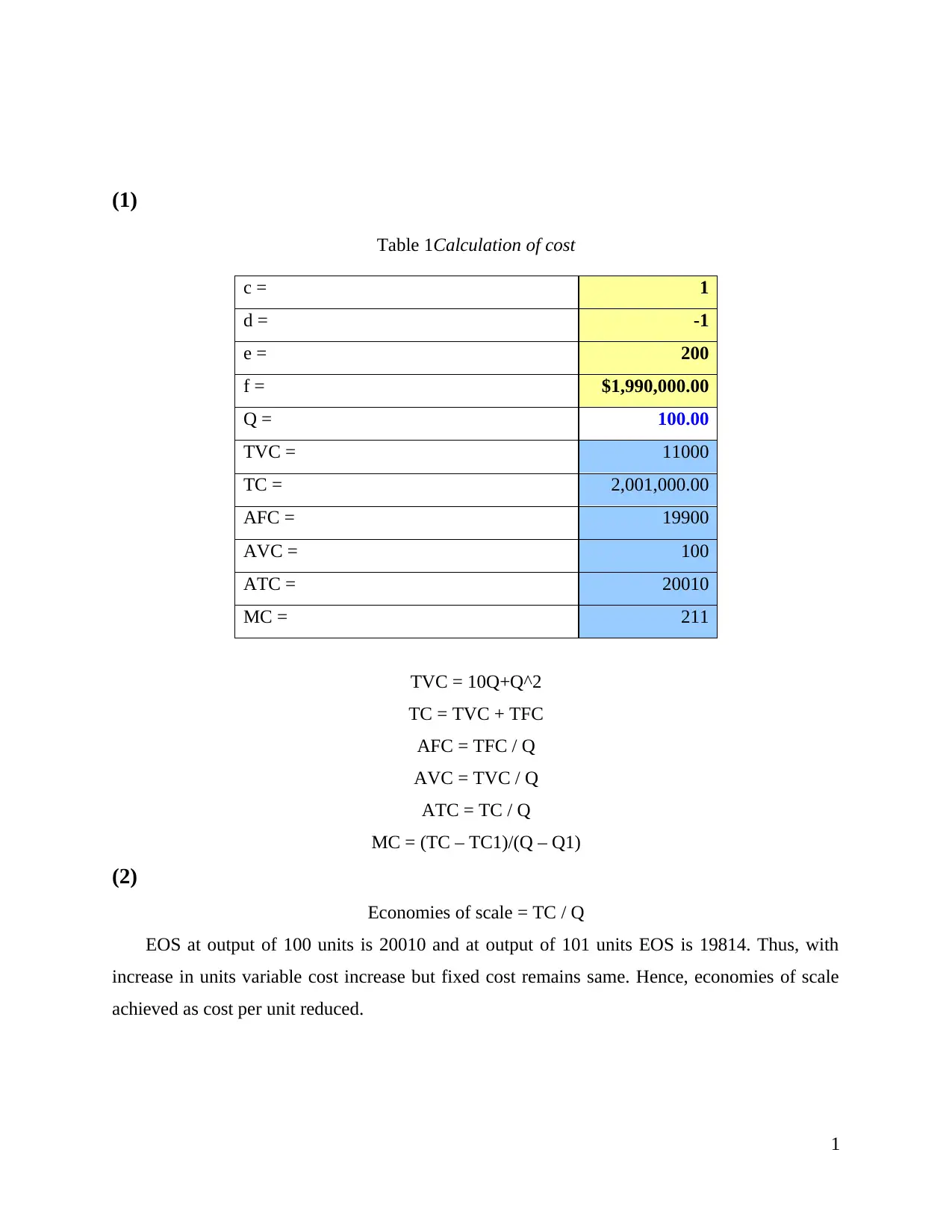
Table 1Calculation of cost
c = 1
d = -1
e = 200
f = $1,990,000.00
Q = 100.00
TVC = 11000
TC = 2,001,000.00
AFC = 19900
AVC = 100
ATC = 20010
MC = 211
TVC = 10Q+Q^2
TC = TVC + TFC
AFC = TFC / Q
AVC = TVC / Q
ATC = TC / Q
MC = (TC – TC1)/(Q – Q1)
(2)
Economies of scale = TC / Q
EOS at output of 100 units is 20010 and at output of 101 units EOS is 19814. Thus, with
increase in units variable cost increase but fixed cost remains same. Hence, economies of scale
achieved as cost per unit reduced.
1

(3)
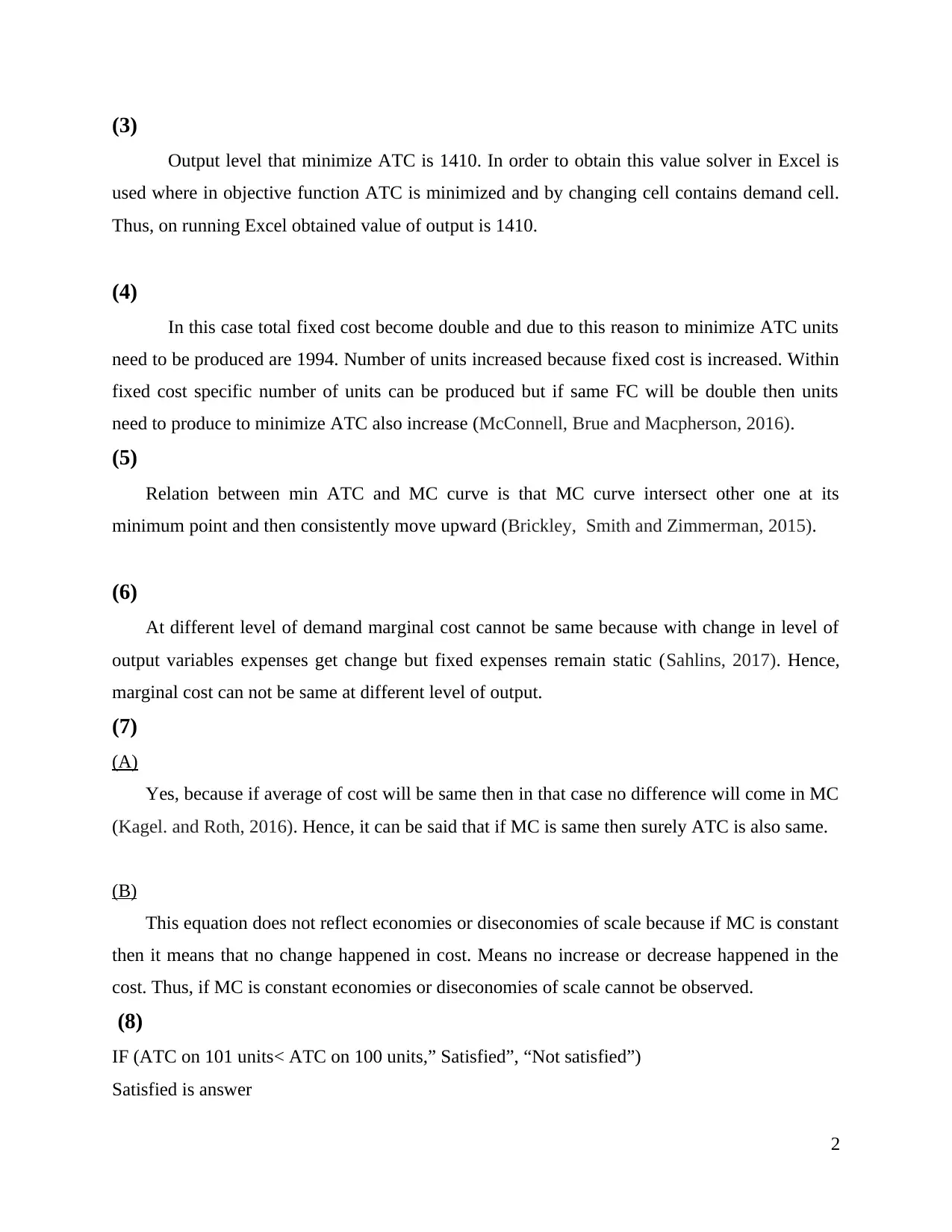
Output level that minimize ATC is 1410. In order to obtain this value solver in Excel is
used where in objective function ATC is minimized and by changing cell contains demand cell.
Thus, on running Excel obtained value of output is 1410.
(4)
In this case total fixed cost become double and due to this reason to minimize ATC units
need to be produced are 1994. Number of units increased because fixed cost is increased. Within
fixed cost specific number of units can be produced but if same FC will be double then units
need to produce to minimize ATC also increase (McConnell, Brue and Macpherson, 2016).
(5)
Relation between min ATC and MC curve is that MC curve intersect other one at its
minimum point and then consistently move upward (Brickley, Smith and Zimmerman, 2015).
(6)
At different level of demand marginal cost cannot be same because with change in level of
output variables expenses get change but fixed expenses remain static (Sahlins, 2017). Hence,
marginal cost can not be same at different level of output.
(7)
(A)
Yes, because if average of cost will be same then in that case no difference will come in MC
(Kagel. and Roth, 2016). Hence, it can be said that if MC is same then surely ATC is also same.
(B)
This equation does not reflect economies or diseconomies of scale because if MC is constant
then it means that no change happened in cost. Means no increase or decrease happened in the
cost. Thus, if MC is constant economies or diseconomies of scale cannot be observed.
(8)
IF (ATC on 101 units< ATC on 100 units,” Satisfied”, “Not satisfied”)
Satisfied is answer
2

REFERENCES
Books and Journals
Brickley, J., Smith, C. and Zimmerman, J., 2015. Managerial economics and organizational
architecture. McGraw-Hill Education.
Kagel, J.H. and Roth, A.E. eds., 2016. The handbook of experimental economics (Vol. 2).
Princeton university press.
McConnell, C., Brue, S. and Macpherson, D., 2016. Contemporary labor economics. McGraw-
Hill Education.
Sahlins, M., 2017. Stone age economics. Routledge.
3