Modeling Velocity of a Skydiver

This assignment explores the dynamics of skydiving by analyzing Felix Baumgartner's freefall. Students are tasked with developing a mathematical model for his velocity, considering factors like gravity and air resistance. The model utilizes differential equations and graphical representations to predict his velocity at various points during the descent. Additionally, students evaluate the strengths and limitations of different velocity models used in this scenario.

Velocity Models 1
Calculus and Velocity Models
Author
Professor
University
City, State
Date

Velocity Models 2
Calculus and Velocity Models
1. Use calculus to model the velocity as a function of time
The velocity, distance and acceleration of an object falling from space are all
connected since the derivative of t he distance yield the instantaneous velocity of the while the
derivative of velocity yields the instatabeoius acceleration at a given point. Since the derivative
and finding the indefinite integral are reverse actions to each other, velocity as a function of time
can be established through finding the indefinite integral of a an acceleration as the function of
time.
a ( t )=∫ v ( t ) . dt
v ( t )=∫ s ( t ) . dt
a ( t ) =∫−1342 ( t ) . dt
a ( t ) =∫−1342 t+ c
At a t=42s
V=1342
At t=0. V=0
But at vo = c1
Thus v ( t )=−1342 t+vo
And s ( t )=−671 t2
t + vo+s
Use integration to determine the expression for the velocity as a function of time
1. In the first 42 seconds of Felix Baumgartner’s fall, the only 2 forces acting on him as he
skydived are the gravitation pull of the earth which made him fall and the air resistance

Velocity Models 3
which had a tendency of pushing him upwards, against gravity From the physics of
projection, the velocity of the jump can be expressed in graphical manner. Since the first
42 seconds entail his jumping from outside of space, the air resistance tends to vary with
the speed of his mass falling from all the way in space. At the same time the impact of
gravity remains constant throughout his entire jump. The jumper will thus experience an
external force acting on his body that will vary the speed of the fall for the first 42
seconds. Because of this variation, a calculus model is the best mathematical tool to
express the variation between the velocity and time is a calculus model. This external
force can be established by obtaining the difference between the gravitational forces and
the air resistance , which will also vary with the difference in time.
F ( t ) =Fg ( t ) −FAR (t)
The constant gravitational forces that the jumper experiences during the time can be
obtained by the formula:
g ( t )= GM
r (t ' )
Where G = gravitational constant between the space and the earth’s surface and
R = radius
M = is the mass.
The value of G is 6.67 x 10-11 m3 kg-1 s-2
And the mass of planet Mars is 639 x 1021 kg
And the radius of Mars is 3390 km. This radius continues to vary during the fall as the body of
the jumper approaches earth and the distance is reduced.
The g obtained which is the initial acceleration is 3.63m/s2
The force of acceleration can be given by the 2 formula of force,

Velocity Models 4
m y'' =−mg
The aspects of distance and velocity have been taken into consideration in this formula to bring
out the relationship between force and time is clearly brought about when the varying force of
the air resistance has been ignored. (Collino, et al., 2014)The resultant force can also be
calculated as being related to the air resistance drag calculated using the formula:
f drag= 1
2 AKρ v2
Thus considering the calculus between velocity and time, the combination of the forces the
jumper experiences can be summed up using the formula:
m y'' =−mg+ 1
2 AKρ( y) y2
Integrating,
m ( ∬s ( t ) .dt ) =−mg+ 1
2 AKρ∫ s ( t ) . dt
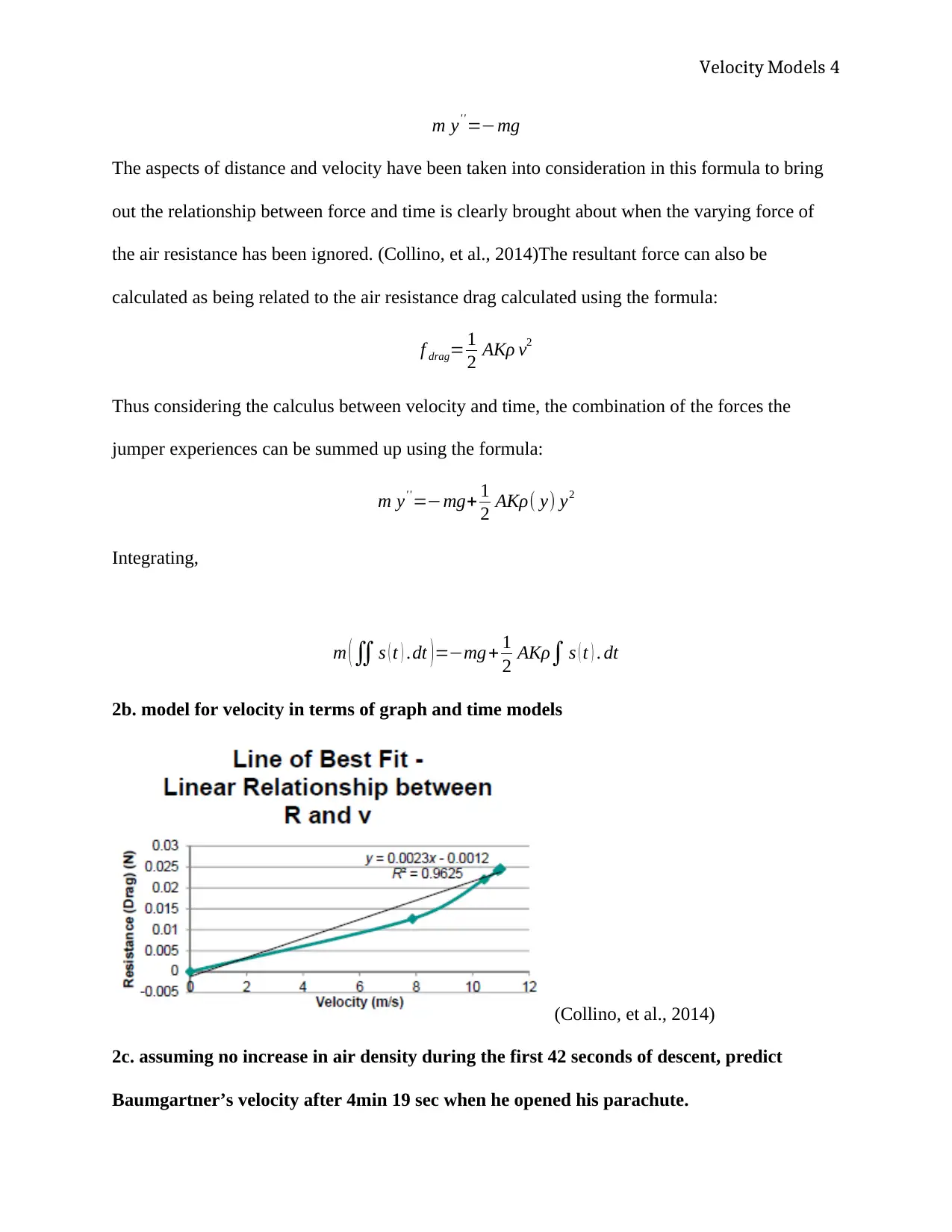
2b. model for velocity in terms of graph and time models
(Collino, et al., 2014)
2c. assuming no increase in air density during the first 42 seconds of descent, predict
Baumgartner’s velocity after 4min 19 sec when he opened his parachute.

Velocity Models 5
vsound =331.3+0.606 t m/ s
The average acceleration is given by
afall=
−410 m
s
42 s = 9.76 m
s
9.76m/s2 = -1342 ( 422/42) + a0
A=f(t)/m
A0=3.76
V= at a t=4min 19s= 376s
v ( t ) =∫ s ( t ) . dt
v ( t ) =∫ ( t ) . dt
v ( t ) =∫ s(¿ 376)+c ¿
v ( 0 )=−475m/s
V(376) = -274m/s
3a. suitable differential equation for the velocity of the jump for the first 42 seconds
∫ dx
a2 −x2 = 1
2 a ln a+ x
a−x +c
And R=−mg +k v2
f =ma=m ( dv
dt )=−mg+k v2
A=-g+k/m( 1
2 a ln a+ x
a− x +c)
V=274.78m/s (Collino, et al., 2014)
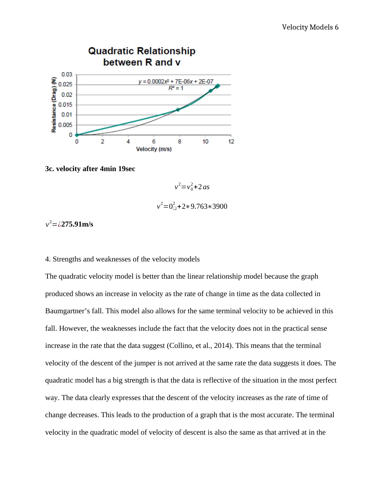
3b.

Velocity Models 6
3c. velocity after 4min 19sec
v2=v0
2 +2 as
v2=0❑
2 +2∗9.763∗3900
v2=¿275.91m/s
4. Strengths and weaknesses of the velocity models
The quadratic velocity model is better than the linear relationship model because the graph
produced shows an increase in velocity as the rate of change in time as the data collected in
Baumgartner’s fall. This model also allows for the same terminal velocity to be achieved in this
fall. However, the weaknesses include the fact that the velocity does not in the practical sense
increase in the rate that the data suggest (Collino, et al., 2014). This means that the terminal
velocity of the descent of the jumper is not arrived at the same rate the data suggests it does. The
quadratic model has a big strength is that the data is reflective of the situation in the most perfect
way. The data clearly expresses that the descent of the velocity increases as the rate of time of
change decreases. This leads to the production of a graph that is the most accurate. The terminal
velocity in the quadratic model of velocity of descent is also the same as that arrived at in the

Velocity Models 7
real sense. This is also true for the slope of the curve which also is the same that of the data
collect. The weakness of this model however predicts values of the model that are negative
which are impossible in the case of the jumper’s descent onto earth (Collino, et al., 2014).

Velocity Models 8
References
Collino, J., Barbero, A. J. & Tapiador, F. J., 2014. Dynamics of a skydiver's freefall. Physics,
15(9), pp. 64-65.