CAPM Modeling Problems - Desklib

This article discusses the risk and return analysis of two stocks, Boeing (BA) and GD, using CAPM modeling. Descriptive statistics and Jarque-Berra test were performed to evaluate the normality of the samples. T-test and F-test were used to compare the average return and risk of the two stocks. The article provides expert guidance on solving CAPM modeling problems.

CAPM Modeling Problems
Student Name: Student ID:
Unit Name: Unit ID:
Date Due: Professor Name:
12

Answer 1: The returns of the two stocks, respectively Boeing (BA) and GD have calculated
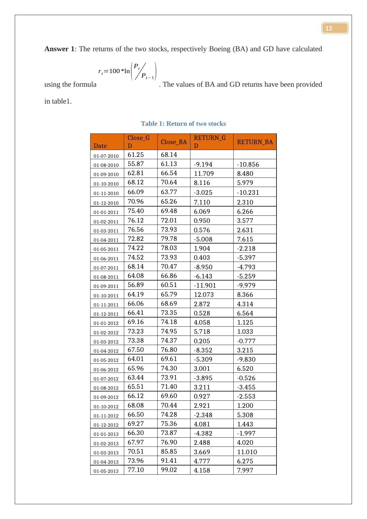
using the formula
rt=100 *ln ( Pt
Pt −1 ) . The values of BA and GD returns have been provided
in table1.
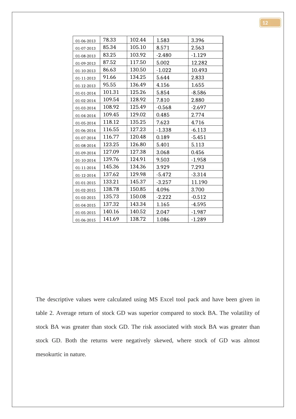
Table 1: Return of two stocks
Date
Close_G
D Close_BA RETURN_G
D RETURN_BA
01-07-2010 61.25 68.14
01-08-2010 55.87 61.13 -9.194 -10.856
01-09-2010 62.81 66.54 11.709 8.480
01-10-2010 68.12 70.64 8.116 5.979
01-11-2010 66.09 63.77 -3.025 -10.231
01-12-2010 70.96 65.26 7.110 2.310
01-01-2011 75.40 69.48 6.069 6.266
01-02-2011 76.12 72.01 0.950 3.577
01-03-2011 76.56 73.93 0.576 2.631
01-04-2011 72.82 79.78 -5.008 7.615
01-05-2011 74.22 78.03 1.904 -2.218
01-06-2011 74.52 73.93 0.403 -5.397
01-07-2011 68.14 70.47 -8.950 -4.793
01-08-2011 64.08 66.86 -6.143 -5.259
01-09-2011 56.89 60.51 -11.901 -9.979
01-10-2011 64.19 65.79 12.073 8.366
01-11-2011 66.06 68.69 2.872 4.314
01-12-2011 66.41 73.35 0.528 6.564
01-01-2012 69.16 74.18 4.058 1.125
01-02-2012 73.23 74.95 5.718 1.033
01-03-2012 73.38 74.37 0.205 -0.777
01-04-2012 67.50 76.80 -8.352 3.215
01-05-2012 64.01 69.61 -5.309 -9.830
01-06-2012 65.96 74.30 3.001 6.520
01-07-2012 63.44 73.91 -3.895 -0.526
01-08-2012 65.51 71.40 3.211 -3.455
01-09-2012 66.12 69.60 0.927 -2.553
01-10-2012 68.08 70.44 2.921 1.200
01-11-2012 66.50 74.28 -2.348 5.308
01-12-2012 69.27 75.36 4.081 1.443
01-01-2013 66.30 73.87 -4.382 -1.997
01-02-2013 67.97 76.90 2.488 4.020
01-03-2013 70.51 85.85 3.669 11.010
01-04-2013 73.96 91.41 4.777 6.275
01-05-2013 77.10 99.02 4.158 7.997
12

01-06-2013 78.33 102.44 1.583 3.396
01-07-2013 85.34 105.10 8.571 2.563
01-08-2013 83.25 103.92 -2.480 -1.129
01-09-2013 87.52 117.50 5.002 12.282
01-10-2013 86.63 130.50 -1.022 10.493
01-11-2013 91.66 134.25 5.644 2.833
01-12-2013 95.55 136.49 4.156 1.655
01-01-2014 101.31 125.26 5.854 -8.586
01-02-2014 109.54 128.92 7.810 2.880
01-03-2014 108.92 125.49 -0.568 -2.697
01-04-2014 109.45 129.02 0.485 2.774
01-05-2014 118.12 135.25 7.623 4.716
01-06-2014 116.55 127.23 -1.338 -6.113
01-07-2014 116.77 120.48 0.189 -5.451
01-08-2014 123.25 126.80 5.401 5.113
01-09-2014 127.09 127.38 3.068 0.456
01-10-2014 139.76 124.91 9.503 -1.958
01-11-2014 145.36 134.36 3.929 7.293
01-12-2014 137.62 129.98 -5.472 -3.314
01-01-2015 133.21 145.37 -3.257 11.190
01-02-2015 138.78 150.85 4.096 3.700
01-03-2015 135.73 150.08 -2.222 -0.512
01-04-2015 137.32 143.34 1.165 -4.595
01-05-2015 140.16 140.52 2.047 -1.987
01-06-2015 141.69 138.72 1.086 -1.289
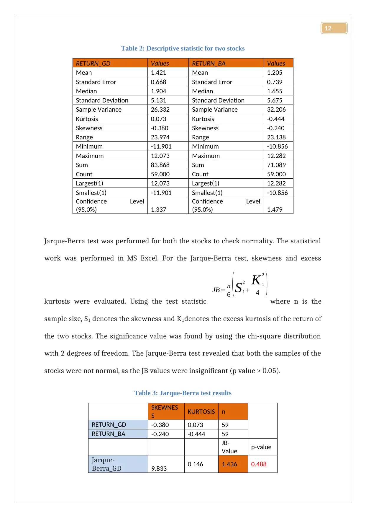
The descriptive values were calculated using MS Excel tool pack and have been given in
table 2. Average return of stock GD was superior compared to stock BA. The volatility of
stock BA was greater than stock GD. The risk associated with stock BA was greater than
stock GD. Both the returns were negatively skewed, where stock of GD was almost
mesokurtic in nature.
12

Table 2: Descriptive statistic for two stocks
RETURN_GD Values RETURN_BA Values
Mean 1.421 Mean 1.205
Standard Error 0.668 Standard Error 0.739
Median 1.904 Median 1.655
Standard Deviation 5.131 Standard Deviation 5.675
Sample Variance 26.332 Sample Variance 32.206
Kurtosis 0.073 Kurtosis -0.444
Skewness -0.380 Skewness -0.240
Range 23.974 Range 23.138
Minimum -11.901 Minimum -10.856
Maximum 12.073 Maximum 12.282
Sum 83.868 Sum 71.089
Count 59.000 Count 59.000
Largest(1) 12.073 Largest(1) 12.282
Smallest(1) -11.901 Smallest(1) -10.856
Confidence Level
(95.0%) 1.337
Confidence Level
(95.0%) 1.479
Jarque-Berra test was performed for both the stocks to check normality. The statistical
work was performed in MS Excel. For the Jarque-Berra test, skewness and excess
kurtosis were evaluated. Using the test statistic
JB= n
6 ( S1
2
+
K1
2
4 ) where n is the
sample size, S1 denotes the skewness and K1denotes the excess kurtosis of the return of
the two stocks. The significance value was found by using the chi-square distribution
with 2 degrees of freedom. The Jarque-Berra test revealed that both the samples of the
stocks were not normal, as the JB values were insignificant (p value > 0.05).
Table 3: Jarque-Berra test results
SKEWNES
S KURTOSIS n
RETURN_GD -0.380 0.073 59
RETURN_BA -0.240 -0.444 59
JB-
Value p-value
Jarque-
Berra_GD 9.833 0.146 1.436 0.488
12

Jarque-Berra_BA 9.833 0.107 1.051 0.591
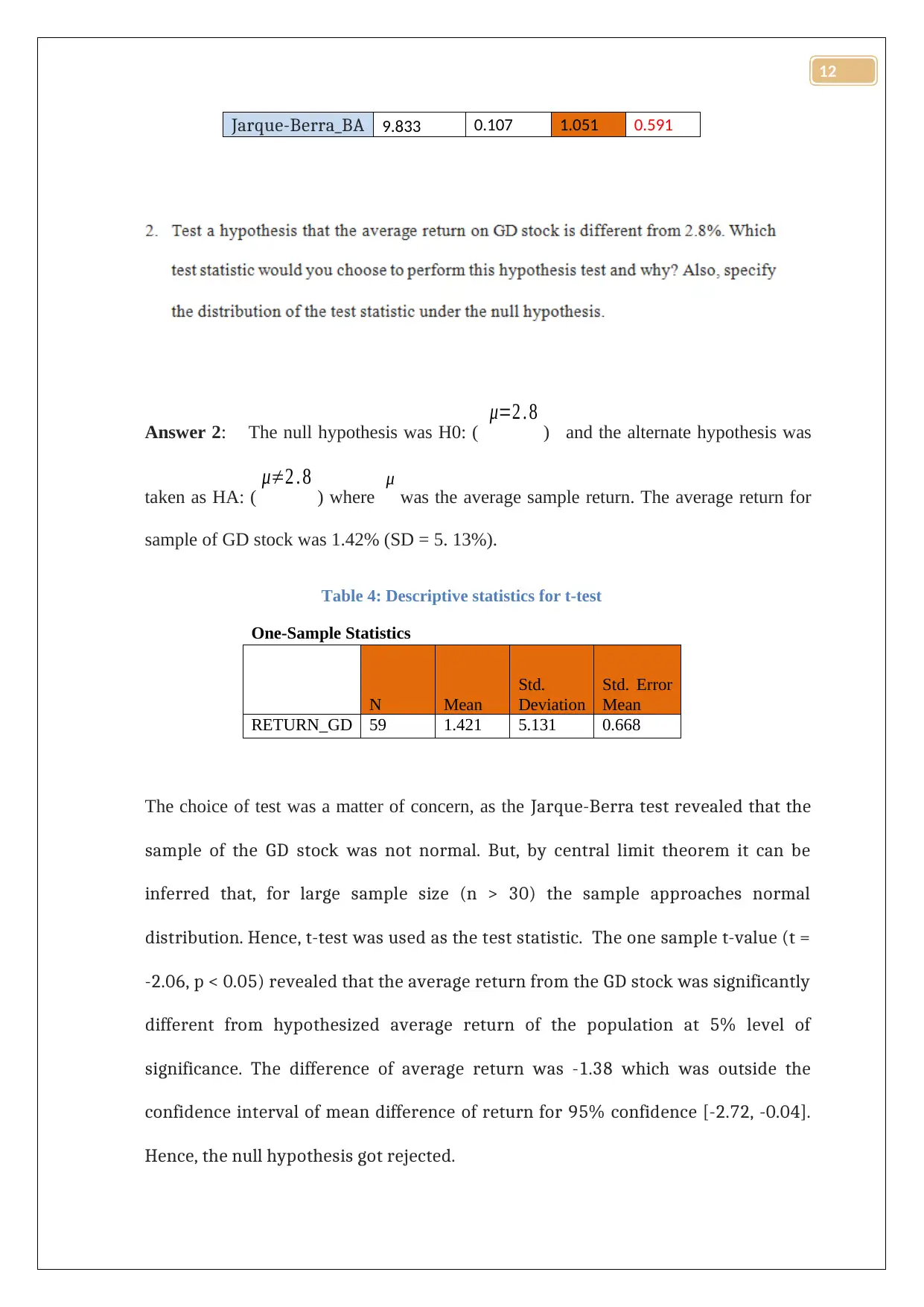
Answer 2: The null hypothesis was H0: (
μ=2 . 8 ) and the alternate hypothesis was
taken as HA: (
μ≠2 . 8 ) where μ
was the average sample return. The average return for
sample of GD stock was 1.42% (SD = 5. 13%).
Table 4: Descriptive statistics for t-test
One-Sample Statistics
N Mean
Std.
Deviation
Std. Error
Mean
RETURN_GD 59 1.421 5.131 0.668
The choice of test was a matter of concern, as the Jarque-Berra test revealed that the
sample of the GD stock was not normal. But, by central limit theorem it can be
inferred that, for large sample size (n > 30) the sample approaches normal
distribution. Hence, t-test was used as the test statistic. The one sample t-value (t =
-2.06, p < 0.05) revealed that the average return from the GD stock was significantly
different from hypothesized average return of the population at 5% level of
significance. The difference of average return was -1.38 which was outside the
confidence interval of mean difference of return for 95% confidence [-2.72, -0.04].
Hence, the null hypothesis got rejected.
12

Table 5: One sample t-test table for average return
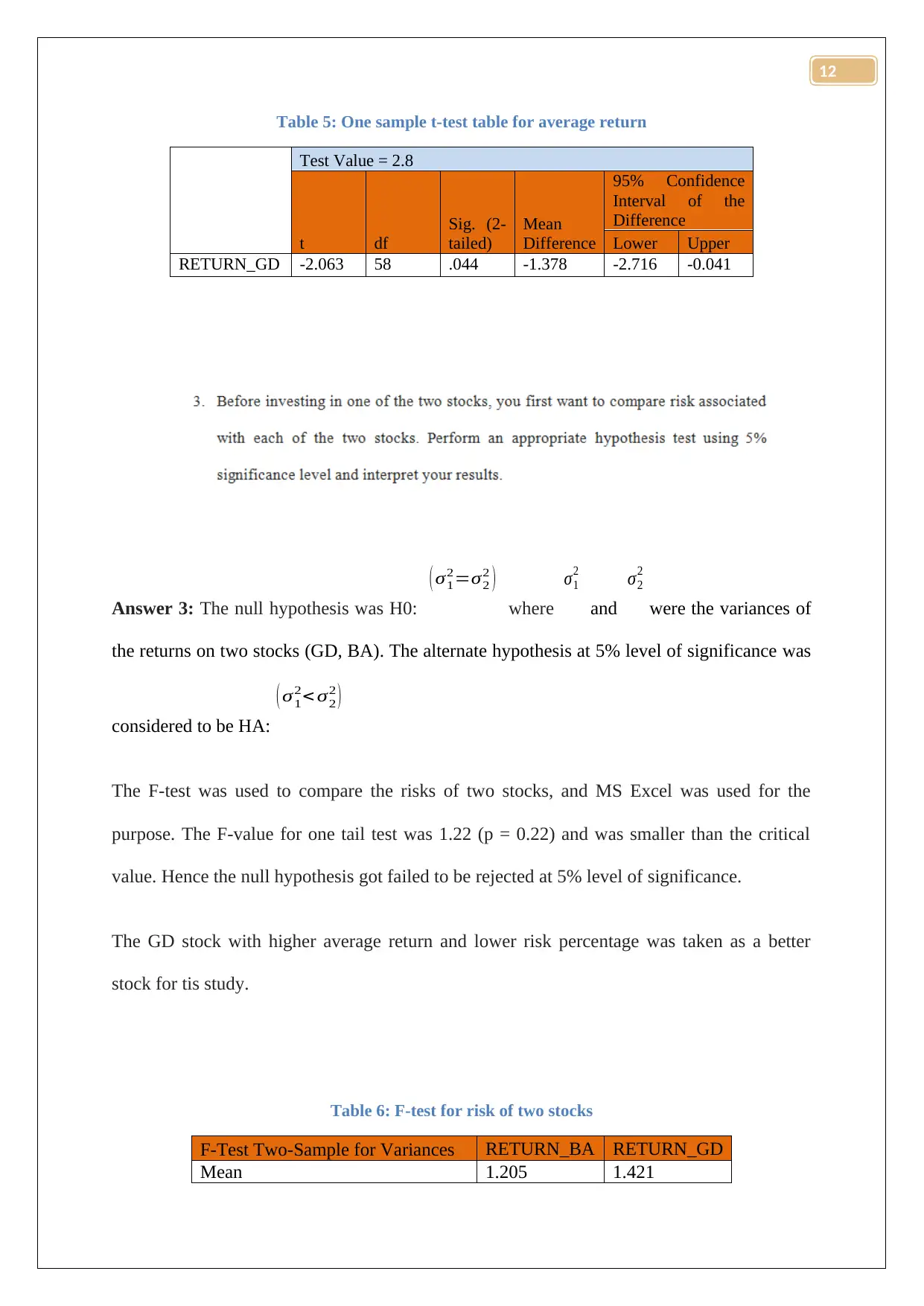
Test Value = 2.8
t df
Sig. (2-
tailed)
Mean
Difference
95% Confidence
Interval of the
Difference
Lower Upper
RETURN_GD -2.063 58 .044 -1.378 -2.716 -0.041
Answer 3: The null hypothesis was H0:
( σ1
2=σ2
2 )
where
σ1
2
and
σ2
2
were the variances of
the returns on two stocks (GD, BA). The alternate hypothesis at 5% level of significance was
considered to be HA:
( σ1
2< σ2
2 )
The F-test was used to compare the risks of two stocks, and MS Excel was used for the
purpose. The F-value for one tail test was 1.22 (p = 0.22) and was smaller than the critical
value. Hence the null hypothesis got failed to be rejected at 5% level of significance.
The GD stock with higher average return and lower risk percentage was taken as a better
stock for tis study.
Table 6: F-test for risk of two stocks
F-Test Two-Sample for Variances RETURN_BA RETURN_GD
Mean 1.205 1.421
12

Variance 32.206 26.332
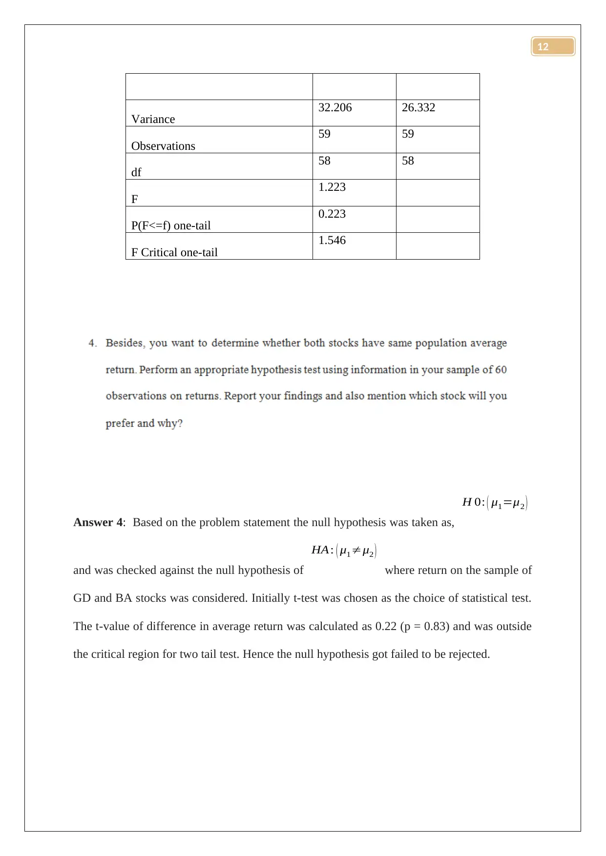
Observations 59 59
df 58 58
F 1.223
P(F<=f) one-tail 0.223
F Critical one-tail 1.546
Answer 4: Based on the problem statement the null hypothesis was taken as,
H 0: ( μ1=μ2 )
and was checked against the null hypothesis of
HA : ( μ1≠μ2 )
where return on the sample of
GD and BA stocks was considered. Initially t-test was chosen as the choice of statistical test.
The t-value of difference in average return was calculated as 0.22 (p = 0.83) and was outside
the critical region for two tail test. Hence the null hypothesis got failed to be rejected.
12

Table 7: T-test of two samples
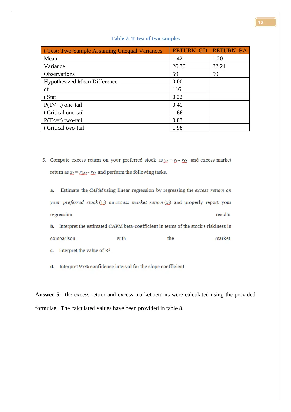
t-Test: Two-Sample Assuming Unequal Variances RETURN_GD RETURN_BA
Mean 1.42 1.20
Variance 26.33 32.21
Observations 59 59
Hypothesized Mean Difference 0.00
df 116
t Stat 0.22
P(T<=t) one-tail 0.41
t Critical one-tail 1.66
P(T<=t) two-tail 0.83
t Critical two-tail 1.98
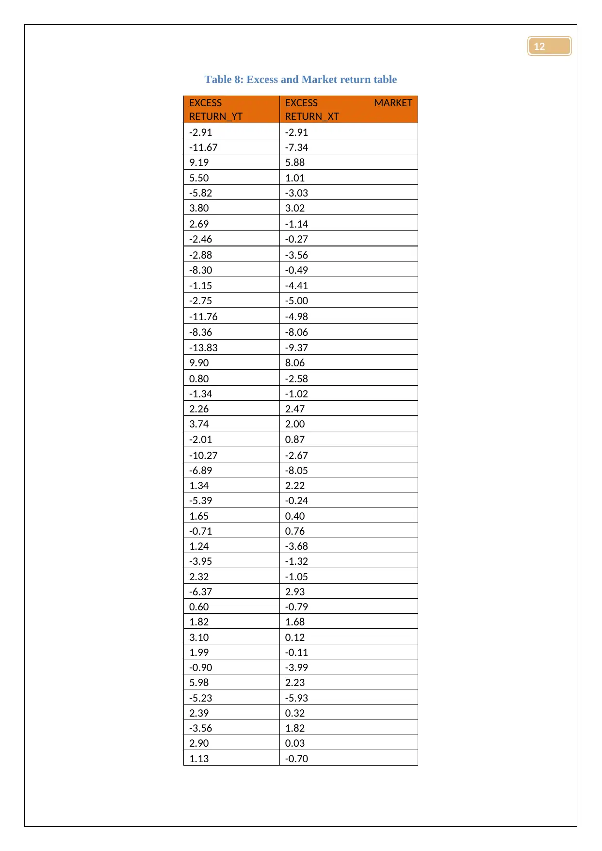
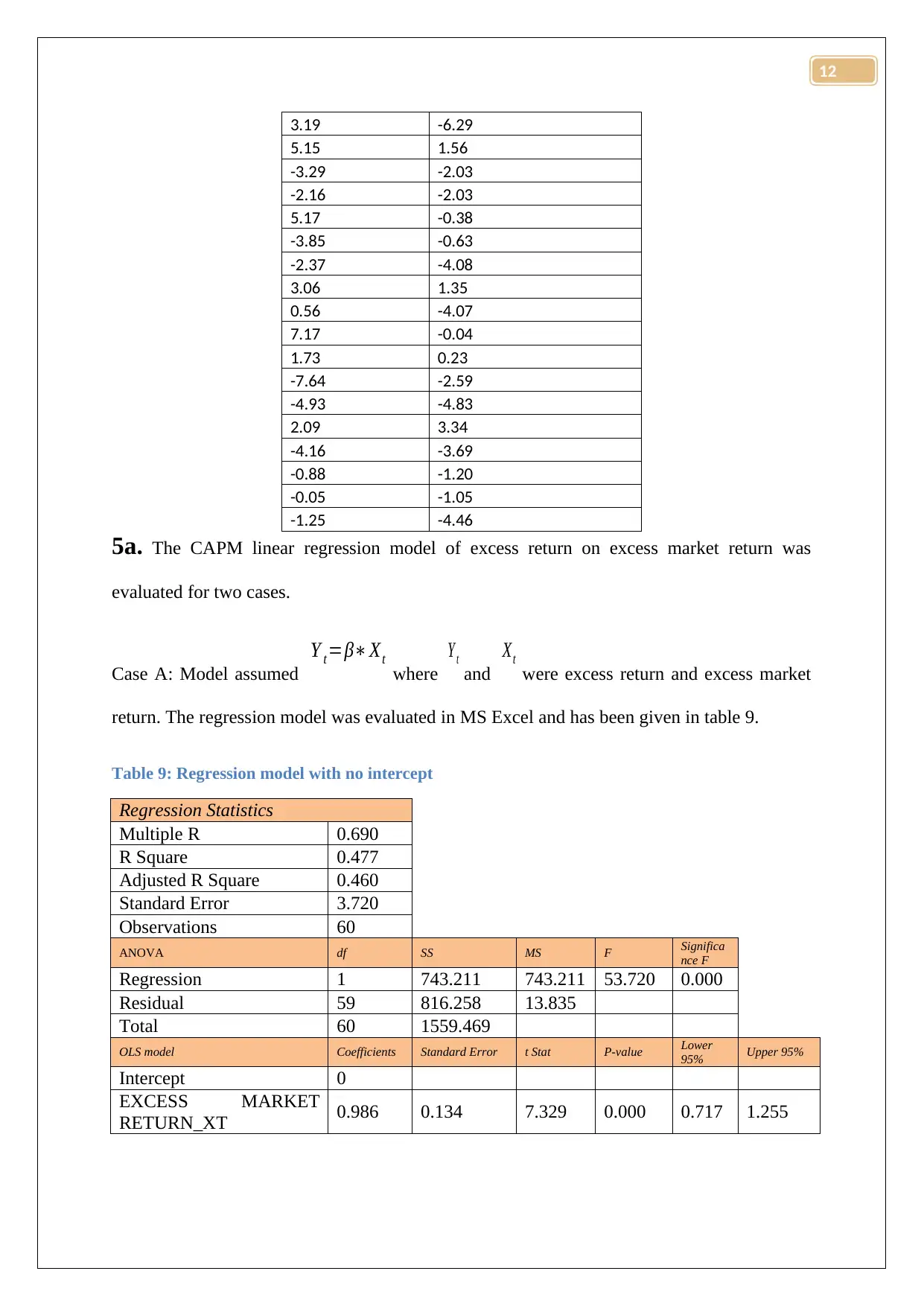
Answer 5: the excess return and excess market returns were calculated using the provided
formulae. The calculated values have been provided in table 8.
12

Table 8: Excess and Market return table
EXCESS
RETURN_YT
EXCESS MARKET
RETURN_XT
-2.91 -2.91
-11.67 -7.34
9.19 5.88
5.50 1.01
-5.82 -3.03
3.80 3.02
2.69 -1.14
-2.46 -0.27
-2.88 -3.56
-8.30 -0.49
-1.15 -4.41
-2.75 -5.00
-11.76 -4.98
-8.36 -8.06
-13.83 -9.37
9.90 8.06
0.80 -2.58
-1.34 -1.02
2.26 2.47
3.74 2.00
-2.01 0.87
-10.27 -2.67
-6.89 -8.05
1.34 2.22
-5.39 -0.24
1.65 0.40
-0.71 0.76
1.24 -3.68
-3.95 -1.32
2.32 -1.05
-6.37 2.93
0.60 -0.79
1.82 1.68
3.10 0.12
1.99 -0.11
-0.90 -3.99
5.98 2.23
-5.23 -5.93
2.39 0.32
-3.56 1.82
2.90 0.03
1.13 -0.70
12

3.19 -6.29
5.15 1.56
-3.29 -2.03
-2.16 -2.03
5.17 -0.38
-3.85 -0.63
-2.37 -4.08
3.06 1.35
0.56 -4.07
7.17 -0.04
1.73 0.23
-7.64 -2.59
-4.93 -4.83
2.09 3.34
-4.16 -3.69
-0.88 -1.20
-0.05 -1.05
-1.25 -4.46
5a. The CAPM linear regression model of excess return on excess market return was
evaluated for two cases.
Case A: Model assumed
Y t=β∗Xt
where
Y t
and
Xt
were excess return and excess market
return. The regression model was evaluated in MS Excel and has been given in table 9.
Table 9: Regression model with no intercept
Regression Statistics
Multiple R 0.690
R Square 0.477
Adjusted R Square 0.460
Standard Error 3.720
Observations 60
ANOVA df SS MS F Significa
nce F
Regression 1 743.211 743.211 53.720 0.000
Residual 59 816.258 13.835
Total 60 1559.469
OLS model Coefficients Standard Error t Stat P-value Lower
95% Upper 95%
Intercept 0
EXCESS MARKET
RETURN_XT 0.986 0.134 7.329 0.000 0.717 1.255
12

The regression CAPM equation was
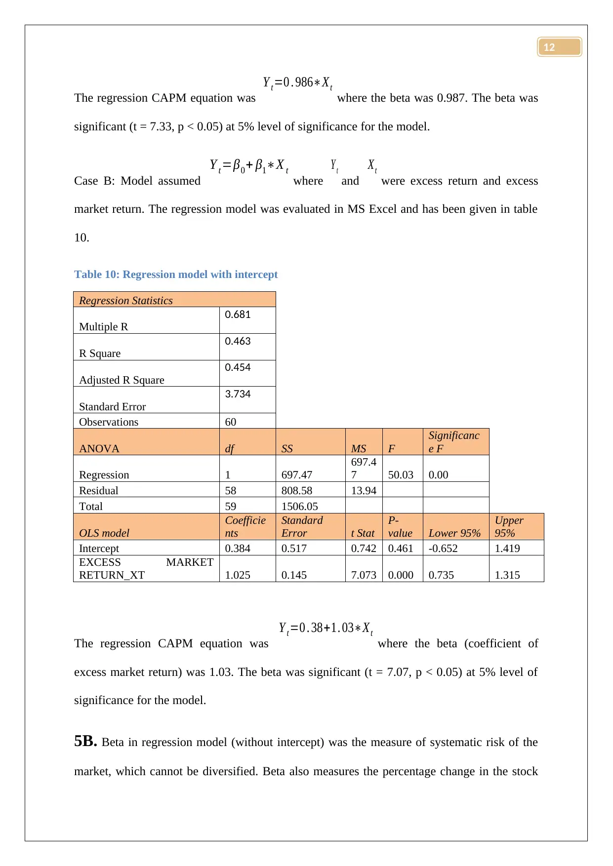
Y t =0 . 986∗Xt
where the beta was 0.987. The beta was
significant (t = 7.33, p < 0.05) at 5% level of significance for the model.
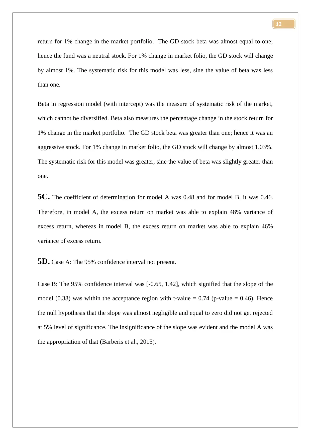
Case B: Model assumed
Y t=β0+ β1∗X t
where
Y t
and
Xt
were excess return and excess
market return. The regression model was evaluated in MS Excel and has been given in table
10.
Table 10: Regression model with intercept
Regression Statistics
Multiple R
0.681
R Square
0.463
Adjusted R Square
0.454
Standard Error
3.734
Observations 60
ANOVA df SS MS F
Significanc
e F
Regression 1 697.47
697.4
7 50.03 0.00
Residual 58 808.58 13.94
Total 59 1506.05
OLS model
Coefficie
nts
Standard
Error t Stat
P-
value Lower 95%
Upper
95%
Intercept 0.384 0.517 0.742 0.461 -0.652 1.419
EXCESS MARKET
RETURN_XT 1.025 0.145 7.073 0.000 0.735 1.315
The regression CAPM equation was
Y t =0 . 38+1. 03∗Xt
where the beta (coefficient of
excess market return) was 1.03. The beta was significant (t = 7.07, p < 0.05) at 5% level of
significance for the model.
5B. Beta in regression model (without intercept) was the measure of systematic risk of the
market, which cannot be diversified. Beta also measures the percentage change in the stock
12

return for 1% change in the market portfolio. The GD stock beta was almost equal to one;
hence the fund was a neutral stock. For 1% change in market folio, the GD stock will change
by almost 1%. The systematic risk for this model was less, sine the value of beta was less
than one.
Beta in regression model (with intercept) was the measure of systematic risk of the market,
which cannot be diversified. Beta also measures the percentage change in the stock return for
1% change in the market portfolio. The GD stock beta was greater than one; hence it was an
aggressive stock. For 1% change in market folio, the GD stock will change by almost 1.03%.
The systematic risk for this model was greater, sine the value of beta was slightly greater than
one.
5C. The coefficient of determination for model A was 0.48 and for model B, it was 0.46.
Therefore, in model A, the excess return on market was able to explain 48% variance of
excess return, whereas in model B, the excess return on market was able to explain 46%
variance of excess return.
5D. Case A: The 95% confidence interval not present.
Case B: The 95% confidence interval was [-0.65, 1.42], which signified that the slope of the
model (0.38) was within the acceptance region with t-value = 0.74 (p-value = 0.46). Hence
the null hypothesis that the slope was almost negligible and equal to zero did not get rejected
at 5% level of significance. The insignificance of the slope was evident and the model A was
the appropriation of that (Barberis et al., 2015).
12

Answer 6: The preferred stock was the GD stock with mean = 1.42%, SD = 5.13%.
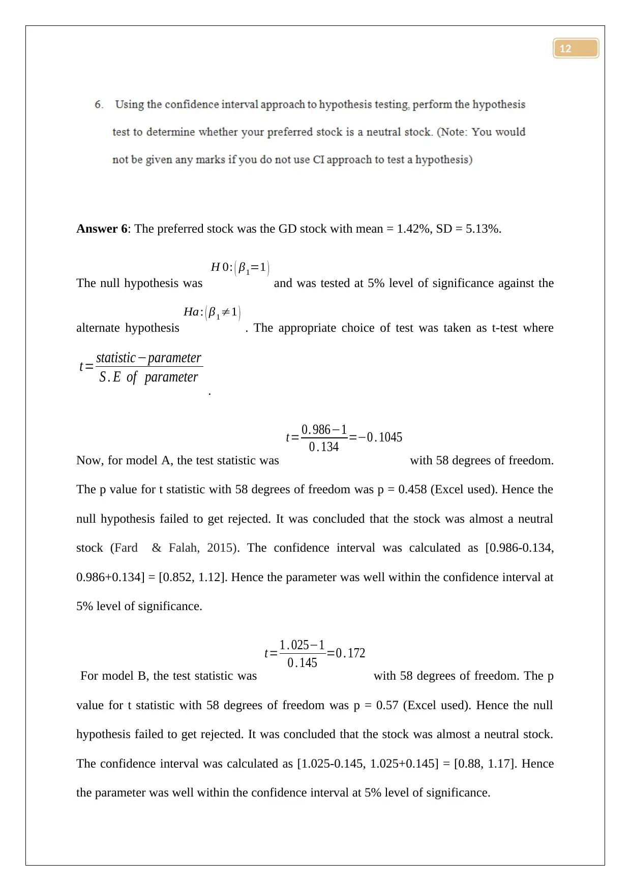
The null hypothesis was
H 0: ( β1=1 ) and was tested at 5% level of significance against the
alternate hypothesis
Ha: ( β1≠1 ) . The appropriate choice of test was taken as t-test where
t = statistic−parameter
S . E of parameter .
Now, for model A, the test statistic was
t= 0. 986−1
0 . 134 =−0 . 1045
with 58 degrees of freedom.
The p value for t statistic with 58 degrees of freedom was p = 0.458 (Excel used). Hence the
null hypothesis failed to get rejected. It was concluded that the stock was almost a neutral
stock (Fard & Falah, 2015). The confidence interval was calculated as [0.986-0.134,
0.986+0.134] = [0.852, 1.12]. Hence the parameter was well within the confidence interval at
5% level of significance.
For model B, the test statistic was
t=1 . 025−1
0 . 145 =0 . 172
with 58 degrees of freedom. The p
value for t statistic with 58 degrees of freedom was p = 0.57 (Excel used). Hence the null
hypothesis failed to get rejected. It was concluded that the stock was almost a neutral stock.
The confidence interval was calculated as [1.025-0.145, 1.025+0.145] = [0.88, 1.17]. Hence
the parameter was well within the confidence interval at 5% level of significance.
12

Answer 7: From the two OLS regression models, standard residuals are plotted in a dot plot.
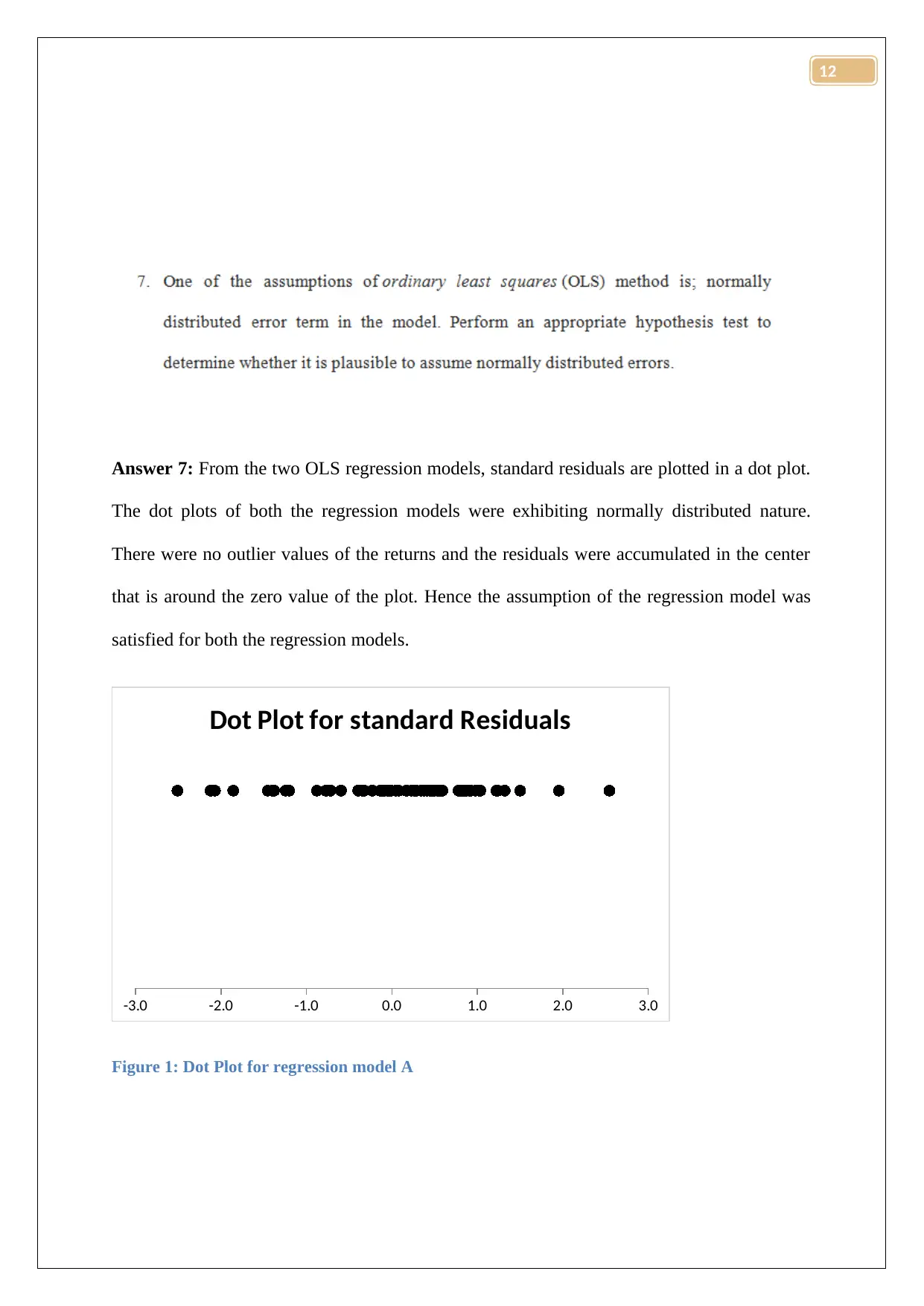
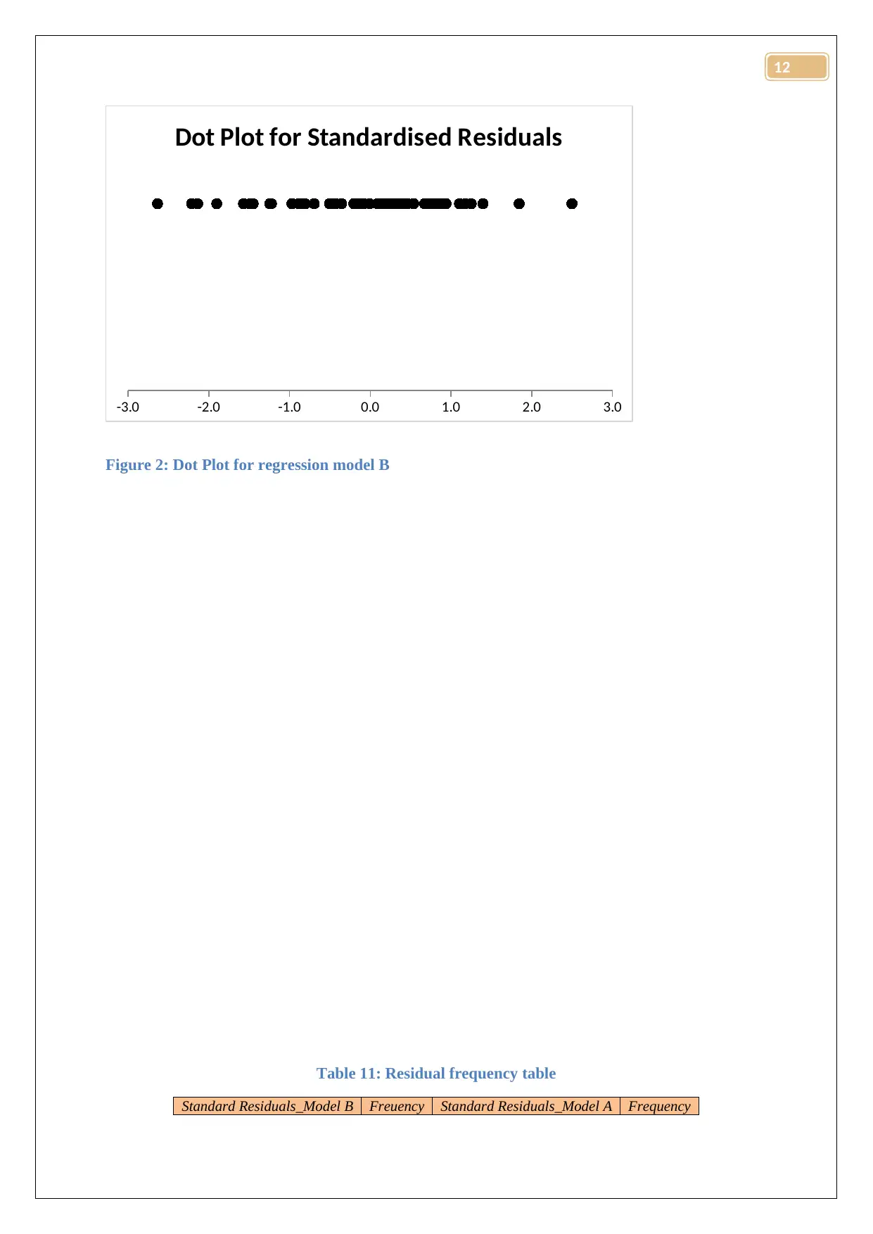
The dot plots of both the regression models were exhibiting normally distributed nature.
There were no outlier values of the returns and the residuals were accumulated in the center
that is around the zero value of the plot. Hence the assumption of the regression model was
satisfied for both the regression models.
-3.0 -2.0 -1.0 0.0 1.0 2.0 3.0
Dot Plot for standard Residuals
Figure 1: Dot Plot for regression model A
12

-3.0 -2.0 -1.0 0.0 1.0 2.0 3.0
Dot Plot for Standardised Residuals
Figure 2: Dot Plot for regression model B
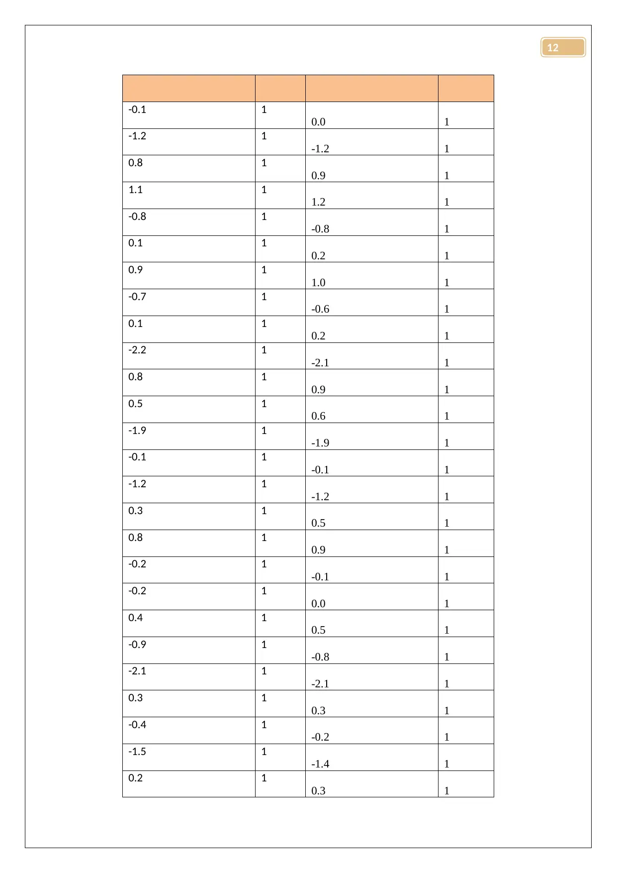
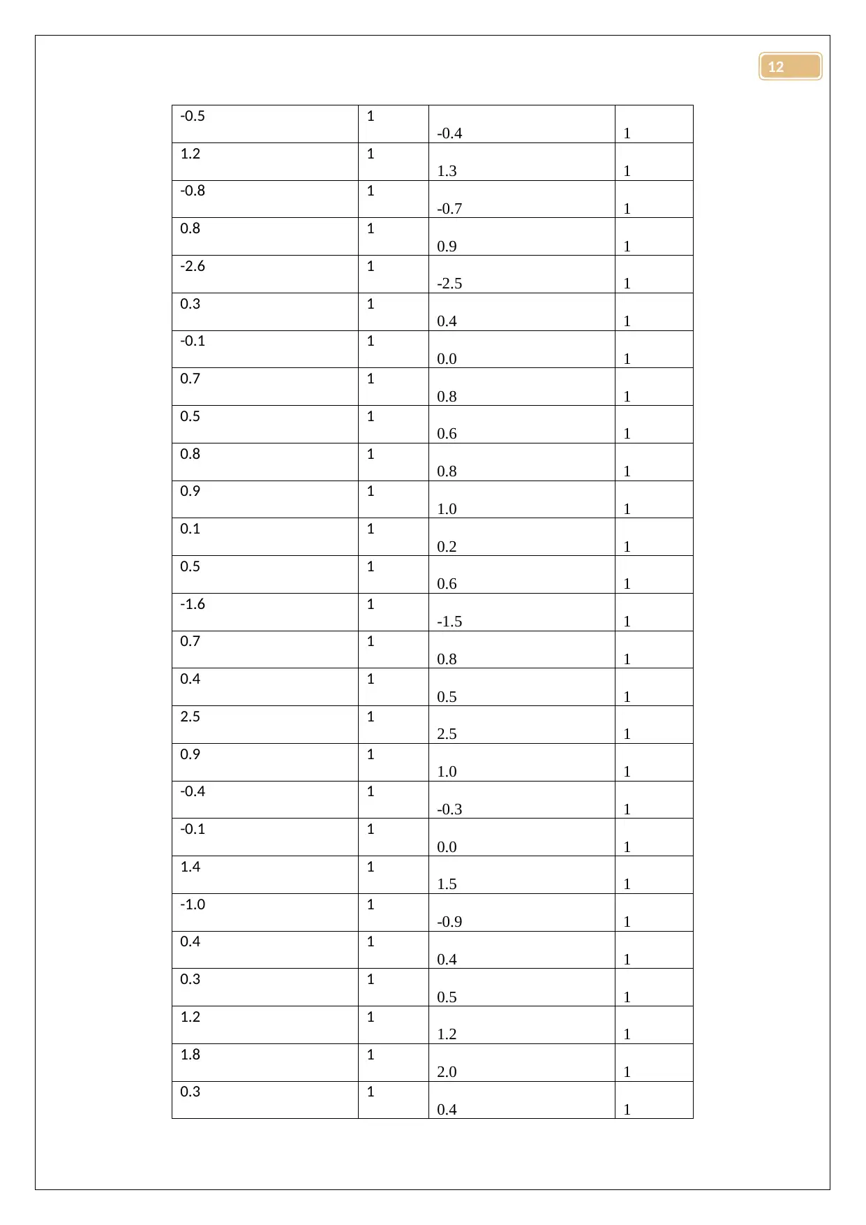
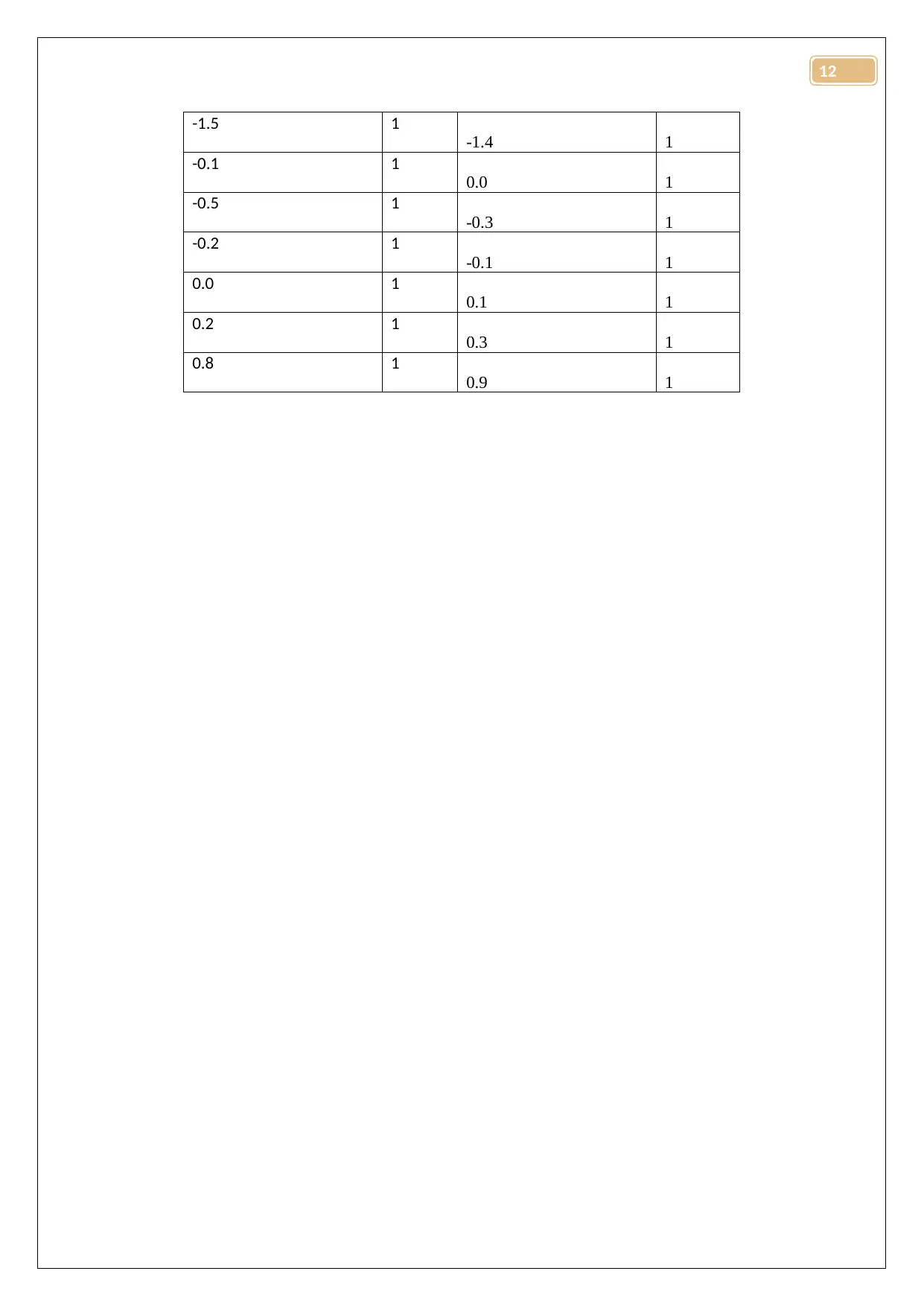
Table 11: Residual frequency table
Standard Residuals_Model B Freuency Standard Residuals_Model A Frequency
12

-0.1 1
0.0 1
-1.2 1
-1.2 1
0.8 1
0.9 1
1.1 1
1.2 1
-0.8 1
-0.8 1
0.1 1
0.2 1
0.9 1
1.0 1
-0.7 1
-0.6 1
0.1 1
0.2 1
-2.2 1
-2.1 1
0.8 1
0.9 1
0.5 1
0.6 1
-1.9 1
-1.9 1
-0.1 1
-0.1 1
-1.2 1
-1.2 1
0.3 1
0.5 1
0.8 1
0.9 1
-0.2 1
-0.1 1
-0.2 1
0.0 1
0.4 1
0.5 1
-0.9 1
-0.8 1
-2.1 1
-2.1 1
0.3 1
0.3 1
-0.4 1
-0.2 1
-1.5 1
-1.4 1
0.2 1
0.3 1
12

-0.5 1
-0.4 1
1.2 1
1.3 1
-0.8 1
-0.7 1
0.8 1
0.9 1
-2.6 1
-2.5 1
0.3 1
0.4 1
-0.1 1
0.0 1
0.7 1
0.8 1
0.5 1
0.6 1
0.8 1
0.8 1
0.9 1
1.0 1
0.1 1
0.2 1
0.5 1
0.6 1
-1.6 1
-1.5 1
0.7 1
0.8 1
0.4 1
0.5 1
2.5 1
2.5 1
0.9 1
1.0 1
-0.4 1
-0.3 1
-0.1 1
0.0 1
1.4 1
1.5 1
-1.0 1
-0.9 1
0.4 1
0.4 1
0.3 1
0.5 1
1.2 1
1.2 1
1.8 1
2.0 1
0.3 1
0.4 1
12

-1.5 1
-1.4 1
-0.1 1
0.0 1
-0.5 1
-0.3 1
-0.2 1
-0.1 1
0.0 1
0.1 1
0.2 1
0.3 1
0.8 1
0.9 1
12

References
Barberis, N., Greenwood, R., Jin, L., & Shleifer, A. (2015). X-CAPM: An extrapolative
capital asset pricing model. Journal of financial economics, 115(1), 1-24.
Fard, H. V., & Falah, A. B. (2015). A New Modified CAPM Model: The Two Beta
CAPM. Jurnal UMP Social Sciences and Technology Management Vol, 3(1).
12