Aerodynamic Design Optimization: A Comprehensive CFD Simulation Report

This report presents a comprehensive overview of Computational Fluid Dynamics (CFD) and its application in aerodynamic design analysis. It begins by outlining the objectives of the simulation, introducing CFD principles, and highlighting its significance in the automotive industry. The methodology adopted for the simulation is detailed, covering aspects such as the computational domain size, meshing of the model, and the engineering database used. The report then discusses the results obtained from the CFD simulation, including advantages and disadvantages of the design, and explores potential future developments. Specific applications of CFD in areas like industrial manufacturing, civil engineering, environmental engineering, and naval architecture are also examined, providing a broad understanding of CFD's versatility. The document concludes with an aerodynamic test, its weaknesses, advantages, suggested improvements, and a comparative discussion of the original and enhanced designs.

CFD
[Document subtitle]
MARCH 13, 2018
HP
[Company address]

Table of Contents
1. Objective of simulation.
2. Introduction to CFD.
3. CFD in automobile and engine applications.
4. Introduction of CFD in fluid dynamics.
5. Aim of the simulation
6. Methodology Adopted
7. Procedure
8. Analysis Environment
9. Size of Computational Domain
10. Meshing the Model
11. Engineering Database
12. Results
13. Advantages of CFD
14. Disadvantages of CFD
15. Future of CFD
II

General Information
1. Objective of the simulation:-Test the car Body in the Environment (aerodynamic) of a car.
Introduction:- In recent years we have seen a rapid increase in the use of computers for engineers in solving
the problems. In the same contrast particularly Computational Fluid Dynamics (CFD) is true subject for the
problem solving that involves fluid heat transfer and fluid flow which occur in applications related
aerospace, power sector and automobile industry. The various factors that are the reasons for the
development of CFD are:-
 Growth in the complexity of the engineering problems that can be unsolved in manual way.
 Need of quick solution with moderate accuracy.
 The expenses that an industry bears during laboratory experiment of physical prototype.
 The absence of analytical solutions.
 Exponential growth in the number crunching abilities and rigorous computer speed and its memory.
[1]
CFD plays a vital role to influence the design of automobile components because of
continuous advancement in computer hardware and software including advancement
in the numerical technique-s in order to derive results from the various equations
which are related to the fluid-flow mechanism. The automobile industry has a keen
interest in CFD. It is considered that CFD contains huge potential to significantly
improve design of the cars and other automobile and at the same time it can reduce
the cost of product and life cycle time and the day came CFD has brought revolution
in field of automotive design. CFD enables us to utilize its tools more in day today
automobile and aircraft design. We can better estimate the conditions for which CFD
applications can be used in the up-coming period of years. CFD applications in the any
industries have large number ofcodes available for designing of any product. There
are several applications in various portions which ranges from system - level (e.g.,
external aerodynamics) to the individual components - level (e.g., cooling system of
disk break). The physics that is associated covering the variety of ranges of flow
regimes like as incompressible flow, laminar flow, compressible flow, turbulent flow,
unsteady flow, steady flow, subsonic flow and transonic flow. A major portion of the
applications of CFD comes under the range which can not be compressed and rest of
those are in the turbulent flows. The fact is most of the flows which can be seen in
reality are actually unsteady type flow in nature but maximum of them can be
adjudged as steady flow cases. Today the major problem is to execute the simulation
1

accurately and precisely some of the complicated thermo-fluids phenomenon’s, and to
be capable of obtaining CFD quicker results to efficiently implement them in the
“dynamic” design scenario of frequently changing designs. The general ideais to use
and utilize CFD in the primary phases of designing in order to fix the design change-s
and to optimize the process. The proper use and implementation of CFD results in
user to more significantly decrease need of doing prototyping and consequently,
reduces cost of design and cycle time associated to it.[2]
2. Introduction to CFD:-
Question: What is CFD? CFD is fundamentally defined as a physical quality of any fluid - flow that
is having three governing fundamental principles:-
 Conservation of mass for the fluid.
 Newton’s Second Law :- According to the law “the rate of the change of momentum is
directly proportional to the force applied and this rate of change of momentum is directly
proportional to the applied force and in the direction of the applied force”.
 Law of conservation of energy- The law which, is the first law of thermodynamics and it
states that “the summation of the rate of change of heat addition must be equal to the work
done on the fluid”.
In order to continue the understanding of CFD the person must first understand the fluid dynamics and its
governing equation.
The Computational Fluid Dynamics equations can be derived in two stages.
 First stage is the numerical discretization.
 Second stage is the specific technique.
The above two stages are used to solve the algebraic equations which is derived from
the governing equations.
2.1. Discretization :-Thediscretization process are identified by some
fundamental processes that we are still using now a days. The two most
common methods are the finite-element and spectral methods.
2.1.1. Finite Element Method
The finite element method is the oldest method among all methods which are applied
in solving the numerical solution derived from partial differential equations. This
method was derived by a famous scientist Euler in year 1768. This method is applied
to obtain numerical solutions ofthe differential equations by manual calculating it i.e.
2

by hand calculation. In this methodat a number of grids/elements are defined with
their respective nodal points. Each grid with the number of nodal points are used in
order to demonstrate the particular domain of fluid - flow. Thereafter the concept of
Taylor series expansion is applied in-order to generate finite type of difference
approximation-s to the partial derivatives of the equations which govern. These
derivatives are then alternated by using finite-difference approximations and theseall
results in forming an algebraic equation which describes the flow solution at each of
the grid point. This method is most commonly used in grids which are structured as it
just takes a mesh which contains a high degree of regularity and accuracy. From all
above discussion Finite Element Method can be summarized in three basic features:-
1. Bifurcate the whole body / structure into parts, finite element.
2. For each representative elements create the relations among secondary and
primary variable.
3. Assemble of the elements to obtain the relations in form of equation or a matrix
between the secondary and primary variables.
As per discretization is concerned the two compatibility conditions must be ensured:-
1. Compatibility of nodal displacement:- When a body is deformed without
breaking, no crack appears in stretching and particles do not penetrates each
other in elements. Such situation is called Nodal displacement compatibility. The
compatibility condition confirms that the displacement is continuous and single
value function of position.
2. Equilibrium of forces:- The equilibrium at the nodal forces must be ensured.
It is a fact that there are ample number of commercial purpose codes and research
codes those are available and they can be employed but the in finite-element
method CFD application is not so much fruitful. But apart from this there is one
method which is in brief same as finite element method and is seems fruitful and
commercially uses all codes and is essentially used by CFD. The method is called
“Finite - Volume Method (FVM)”. The main separating feature is that FVM utilizes
straightforward piecewise polynomial capacities for nearby elements which has a
tendency to portray the varieties of the unknown stream factors. The weighted
residial idea is acquainted all together to do the assessment of the mistakes
related with the estimated capacities, which are later without a doubt limited. An
arrangement of non-direct mathematical conditions for the obscure terms of the
approximating capacities is solved, subsequently bringing about the stream
3

arrangement. The leftover capacities are explained and the stream arrangements
are obtained by, Collocation technique, Galerkin’s method, Sub-domain technique,
and least square method.
Spectral method
Spectral method has a fundamental approach which is same as that of the finite-
difference and finite-element methods, where the unknown factors of the
equations that are governed are changed with some short series.The difference lies
is in only the method which is implemented. The two prior methods uses local
approximations where as in the contradiction the spectral method implements
global approximation. That is by means of Fourier series, Legendre polynomials, for
the whole domain of the flow. The conflict between the exact solution and the
approximate solution is handled by using a weighted residuals concept which is
almost same as of the finite-element method.
Computational Fluid Dynamics can be defined as a procedure of replacing the partial or the integral
derivatives which are used in the equations with discrete algebraic forms, which are calculated to get
specific values for the fluid flow field values at some discrete points in time or space. At the end of it as a
result, the product of CFD will have a series of numerical values, in contradiction to a closed form analytical
solution. However, as long term result of it, the principle aim of most of the analysis done in engineering
analyses, closed type of analyses or otherwise, is a quantitative illustration of the problem statement, i.e.,
numbers.
The apparatus which has allowed the applied advance of CFD contains a high speed computer with great
efficiency. CFD solutions mainly requires the repetitive abetment of thousands or even up to some millions
of digits, an assignment that is absurd for any person after the aid of a high performance computer.
Therefore, advance in CFD, and its applications to problems of added detail and sophistication, are carefully
accompanying to advances in computer hardware, decidedly in attention to accumulator and beheading
speed. This is why the arch force active the development and construction of high speed new
supercomputers are advancing from CFD set.
Computational Fluid Dynamics is basically defined as a process of analysis of such systems that includes
fluid flow, transfer of heat and some otherphenomenon related to it such as some chemical reactions which
can be shown by the means computer simulations. It can be also the by-product of Computational
Continuum Mechanics which is the primary numerical simulation technology which is identical and is used
for many combination of similar partial differential equations such as
 Numerical stress analysis,
4

 Electromagnetics that includes the low-frequency and high-frequency phenomenon.
 Weather prediction and global oceanic circulation models.
 Some arrangements such as star formation and galactic dynamics.
 Heat and mass transfer systems.
 interaction systems of the structure of fluid.
Applications of CFD are:-
 Automobile and engine applications.
 Industrial Manufacturing Applications:- Considering an example of a mould which is filled with a
molten cast iron. The flow field of molten cast iron is the function of time and is fundamentally
solved as a function of time. The molten cast iron is fed into cavity by both side gating system from
the right, one from the centre and other from the lower part of the mould. The CFD resultsthe three
values of time during filling process:
1. An early time which is the time just after two gates are made open.
2. A time slightly after the two streams surge into cavity.
3. Yet a later time when the two streams imping on oneanother.
These calculations are made by Mampaey and Xu at WTCM Foundry Research centre in Belgium.[10]
 Civil Engineering Applications :- Problems those are related to the rheology of rivers, estuaries,
ponds, lakes etc. are also the major subject of analysis using CFD. One of the most common example
is the pumping of mud out of an underwater mud capture reservoir. Here, a layer of water sits on top
of a layer of mud, and portion of mud is trapped and is being sucked away at the bottom. The
velocity field in both water and mud at certain instant can be calculated using CFD.
 Environmental Engineering Applications:- The subjects of heating, air conditioning and circulation
of air through buildings are all included under the spell CFD.
 Naval Architecture Applications-Submarine :- CFD is a major tools in the filed of hydrodynamic
related problems associated with ships, submarine, torpedos, etc. Considering an example of a CFD
applications to submarine. The calculations were made by Science Applications International
Corporation(SAIC) and were provided by Dr. Nils Salveson of SAIC. The multi-zonal grid used for
the calculation of flow over a common submarine framework. The three dimensional equation
known as Navier Stokes equations for an incompressible type of flow are solved, including a
turbulence model, for the flow over this submarine.
3. CFD in Automobile and Engine Applications.
In order to ensure overall improvement of performance of modern sports cars and transportation purpose
trucks the automobile industries has significantly increased accelerated its use of high-technology research
5

and design tools. CFD helps in better understanding for automobile engineers to precisely understand the
physical flow processes, and in turn to design improved vehicles. [3]
CFD is used in automobile industries by the following ways:-
 Internal combustion engine in-cylinder simulations.
 Prediction of lift and drag coefficient of the body of a car.
 Completion of internal combustion engine components such as air intake, turbo-charging component,
ports of car engines and valves, in-cylinder flow, exhaust and gas treatment.
 External aerodynamic system.
4. Introduction of CFD in fluid dynamics
Study of motion of the fluid with reference of forces and moments is known as fluid dynamics. In fluid flow
there different types of forces occurs in the flow like viscous forces, gravitational forces, pressure forces,
surface tension forces, eddy forces (turbulent forces) and different type of other forces.
All CFD in one form is based on equations which are governing in nature of dynamics of fluid- the
continuity equation, momentum equations and power equations. These equations talk the physics. basically
the equations are the mathematical statements of 3 fundamental physical concepts upon which all the fluid
dynamics is based totally upon:
 Conservation of mass.
 Newton’s second law i.e. F=ma.
 Conservation of energy.
 During the vehicle in motion when the fluid flows under adverse pressure
condition, fluidlooses its momentum. Near the surface the particles have less
momentum so they looses their momentum fastly. At the point where
momentum of the fluid becomes zero and after which near the surface the fluid
surface the fluid moves under adverse pressure condition i.e. in reverse
direction that point is known as point of separation. It is not compulsory that
separation must be present in adverse pressure condition.
In fluid flow velocity is function of space and time, so the acceleration is the function of space and
time. Space component is known as convective acceleration and time component is known as local
acceleration. During the ANSYS analysis the above acceleration place an important role and help the
engineer to make proper aerodynamic design of the vehicle. This is so because the acceleration and
velocity component are responsible for lift and drag of the vehicle. Improper design leads to create
serious lift of vehicle and this may results in serious accident. Inorder to avoid this impact in the
6

absence of physical prototype graphically the prototype is designed and is tested through computer
itself by the use of ANSYS and employing Computational Fluid Dynamics theory.
Apart from the above concept some terms need to be described which will helps to validate the whole
analysis:-
1. Flow Lines:- Fluid flow can be described by 3 flow lines
 Stream line:- It is an imaginary line or curve drawn in space such that tangent drawn gives
velocity vector i.e. velocity vector and stream line vector coincides. The two streamlines
never intersect each other as well as stream line also never intersects itself because at the
point of intersection there will be two velocity fields which is impossible. So there is no flow
across the streamlines.
 Path line:- The line drawn by tracing the path of single fluid particle at different time
integrals. It is defined on the basis of ‘Langrangian description’.
 Streak line:- It is an instantaneous picture of all fluid particles passing through single point.
NOTE:- For the steady flow all three lines are identical i.e. all three line coincides.
2. Acceleration in fluid motion:- In fluid flow velocity is the function of space and time, so it is evident
that the acceleration is also the function of space and time. Space component is known as convective
acceleration and time component is known as Local acceleration.
3. Iso-surface:-An iso-surface is a three-dimensional(3D)isolineanalog.
It is a surface representing to the purposes of a consistent esteem (e.g. weight, temperature, speed,
thickness) which is inside a volume of room; as such, it is that level arrangement of a persistent capacity
whose area is 3D-space. It is a surface which is characterized by an understood condition.
i.e.
F (x,y,z) = f
where, F is the function of space and f is the constant.
The `Iso-surface' is a representation that is utilized for computation and draw a surface within a
volumetric data field on a 3-D surface corresponding to points with a single scalar value. It is displayed
by data set, iso-value, draw (Points, Shaded Points, Wireframe, or Solid Surface), boundary, step and
size. It is normally visualized by computer graphics. It used as data visualization methods
in computational fluid dynamics (CFD) that helps the engineers to study the
characteristics of fluid flow. It is mostly helpful in design the system related to
aerodynamics such as aircraft wings or the super cars models.
7

4. Contours:- It is an outline representing or bounding the shape or form of
something. It is used for representation of typical response system in other
words we can say it is typical curve line which describes the response system.
5. Circulation:- It is the line integration of tangential component of velocity along
the closed loop. It is the scalar quantity.
6. Vorticity:- It is the mathematical measure of rotationality. It is circulation per unit area. It is wice of
the rotation. The direction of vorticity is as that of rotation.
5. Aim of the simulation
1. To create a precise Computational Fluid Dynamics simulation which is of good quality and of course of a
unique vehicle model and to get crucial data about it.
2. Another aim is, creating quality of CFD simulations of two automotive vehicles (cars) which almost follows
each other to test and understand drag phenomenon.
6. Methodology Adopted
1. For a given problem define the physical boundary.
2. The total volume of the fluid is than divided into discrete cells with uniform or non uniform mesh depending
upon the situation.
3. The defined boundary conditions have specific fluid behaviour.
4. Starting the simulation and the equations is solved at steady state.
5. Postprocessor is thereafter used for analysis and visualization of the results.
7. Procedure
1. Creation of vehicle model without use of spoiler:- A vehicle model is made by considering the
given standards and construction factors. The designed model is of a specified computational domain
by using ANSYS software package.
2. Creation of vehicle model with use spoiler: - The geometry of the vehicle prototype is normalized by
the length from front to rear of the car model.
3. Creation of 3D model in a given computational domain:-In order to construct the vehicle
geometry from the given construction point and thereafter to quell 3D air domain in design model
some assumptions are considered. The assumptions those are generally made are, the car must move
forward with a fixed velocity considered as suppose ‘U’ through the air passing by. On the
contradiction it is therefore interpreted while executing the simulation, in case of the air is moving
towards the car with the equal velocity but the in the opposite direction the car is in stationed
condition. The whole computational domain is completed irrespective to the domain of air.
Therefore, the car is taken inside the fluid domain and matching boundary conditions are assigned.
The car body’s surface: sky, inlet, symmetry plane, side plane, ground, car body, spoiler and outlet.
4. Meshing the model:- Meshing is the most crucial stage for the simulation by the software named
ANSYS. Choosing a suitable mesh is the challenging task as a perfect mesh will provide precise,
meaningful and accurate solution whereas on the contradiction wrong meshing will give inaccurate
or wrong answers and will make the analysis vague. In order to know the turbulence properly all the
mesh should be grid independently. Mesh should be made accordingly as much fine as possible
especially at the boundary layer. On the other hand, greater number of mesh element in the car model
which leads to finer meshing and this will increase the computational cost therefore mesh size mush
be optimized in a controlled manner. Therefore, selecting size of mesh element and applying suitable
8

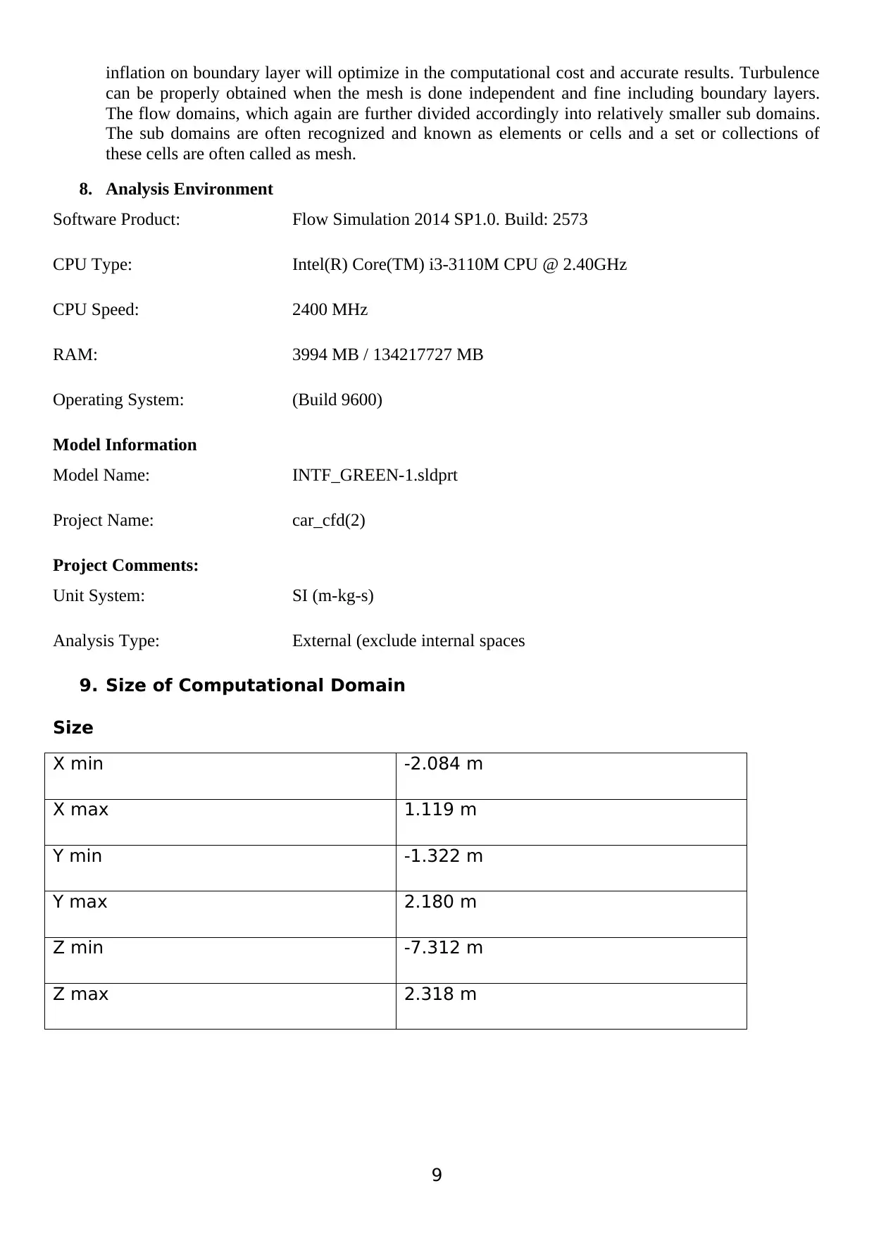
inflation on boundary layer will optimize in the computational cost and accurate results. Turbulence
can be properly obtained when the mesh is done independent and fine including boundary layers.
The flow domains, which again are further divided accordingly into relatively smaller sub domains.
The sub domains are often recognized and known as elements or cells and a set or collections of
these cells are often called as mesh.
8. Analysis Environment
Software Product: Flow Simulation 2014 SP1.0. Build: 2573
CPU Type: Intel(R) Core(TM) i3-3110M CPU @ 2.40GHz
CPU Speed: 2400 MHz
RAM: 3994 MB / 134217727 MB
Operating System: (Build 9600)
Model Information
Model Name: INTF_GREEN-1.sldprt
Project Name: car_cfd(2)
Project Comments:
Unit System: SI (m-kg-s)
Analysis Type: External (exclude internal spaces
9. Size of Computational Domain
Size
X min -2.084 m
X max 1.119 m
Y min -1.322 m
Y max 2.180 m
Z min -7.312 m
Z max 2.318 m
9

Simulation Parameters
Mesh Settings
Basic Mesh
Basic Mesh Dimensions
Number of cells in X 30
Number of cells in Y 50
Number of cells in Z 128
10. Meshing the Model
Analysis Mesh
Total Cell count: 192098
Fluid Cells: 188782
Solid Cells: 1823
Partial Cells: 1493
Trimmed Cells: 0
Additional Physical Calculation Options
Heat Transfer Analysis: Heat conduction in solids: Off
Flow Type: Laminar and turbulent
Time-Dependent Analysis: Off
Gravity: Off
Radiation:
Humidity: Off
Default Wall Roughness: 0 micrometer
Material Settings
Fluids: Air
10

Initial Conditions
Ambient Conditions
Thermodynamic parameters Static Pressure: 101325.00 Pa
Temperature: 293.20 K
Velocity parameters Velocity vector
Velocity in X direction: 0 m/s
Velocity in Y direction: 0 m/s
Velocity in Z direction: -28.000 m/s
Turbulence parameters Turbulence intensity and length
Intensity: 0.10 %
Length: 0.008 m
Goals
Global Goals
GG Normal Force (Z) 2
Type Global Goal
Goal type Normal Force (Z)
Coordinate system Global coordinate system
Use in convergence On
GG Normal Force (Y) 1
Type Global Goal
11

Goal type Normal Force (Y)
Coordinate system Global coordinate system
Use in convergence On
11. Engineering Database
Gases
Air
Path: Gases Pre-Defined
Specific heat ratio (Cp/Cv): 1.399
Molecular mass: 0.0290 kg/mol
Dynamic viscosity
Temperature[K]
Dynamic viscosity[Pa*s]
12

Specific heat (Cp)
Temperature[K]
Specific heat (Cp)[J/(kg*K)]
Thermal conductivity
Analysis Time
Calculation Time: 1074 s
Number of Iterations: 194
13

12. Results
Analysis Goals
Goals
Name Unit Value Progress Use in
converge
nce
Delta Criteria
GG
Normal
Force
(Z) 2
N -13.413 100 On 0.0205115
416
0.428885
13
GG
Normal
Force
(Y) 1
N -5.307 100 On 0.1322407
12
0.135369
716
Global Min-Max-Table
Min/Max Table
Name Minimum Maximum
Pressure [Pa] 100956.99 101951.25
Temperature [K] 293.11 293.59
Density (Fluid)
[kg/m^3]
1.20 1.21
Velocity [m/s] 0 31.454

Velocity (X) [m/s] -19.707 8.659
Velocity (Y) [m/s] -11.901 15.510
Velocity (Z) [m/s] -31.215 0
Temperature (Fluid) [K] 293.11 293.59
Mach Number [ ] 0 0.09
Vorticity [1/s] 1.746e-005 276.745
Shear Stress [Pa] 0 2.45
Relative Pressure [Pa] -368.01 626.25
Heat Transfer
Coefficient [W/m^2/K]
0 0
Surface Heat Flux
[W/m^2]
0 0
Figure 1. Iso View of Wireframe
1

Figure 2.
2
Area of Surface which have
Maximum resistance of Air of
Body
Boundary

Figure 3.
Figure 4.
3

Figure 5.
4
Direction of Air
Direction of Vehicle

13. Advantages of CFD
1. It finds a critical broken process and offers a solution.
2. It involves simplified equations and simulations.
3. Provides better prediction in a short time period.
4. Designs efficiently economical and ensure industry compliance product.
5. Analysis results in design cycles which are shorter in value and industries’ products get to
market faster.
6. CFD is a crucial tool for compressing the design and development cycle allowing for
rapid modeling of automobile.
14. Disadvantages of CFD
1. Initial investment cost is high.
2. Required skilled persons therefore costly in field of professionals.
15. Future of CFD
After the above analysis we have reached a certain platform in understanding of and appreciation
for CFD. CFD is the groundbreakng “third dimension” in the field of fluid dynamics, equally
sharing the stage with the other dimension of pure theory and pure experiment.
CFD has just majorly affected automobile designing, and had turned into the basic innovation for
aerodynamic design throughout the following decade. There is most likely that a noteworthy
focal point of CFD is to upgrade the outline procedure for any machine that arrangements with
liquid.
Today, CFD is widey utilized to calculate complete three dimensional flow fields over the actual
automobiles.
The crucial role played by CFD is that of research, a tool that improves our understanding of the
basic physical nature of fluid dynamics. (K Muralidhar, 2003), (David, 1995) (Katz,
2009) (Atul, 2017) (Simon, 2017)
References
Atul, S., 2017. Introduction to Computational Fluid Dynamics: Development.
West Sussex: John Wiley & Sons Ltd.
5

David, A. J., 1995. Computational Fluid Dynamics. s.l.:McGraw-Hill
international .
K Muralidhar, T. S., 2003. Computational Fluid Flow and Heat Transfer. 2nd
ed. New Delhi: Alpha Science International.
Katz, J., 2009. Race car aerodynamics: Designing for speed. 1rst ed.
California: International Human Powered Vehicle Association.
Simon, M., 2017. Competition Car Aerodynamics. 3rd ed. Poundbury: Veloce
Publishing Ltd, 2017.
Review:
CFD Applications in the Automotive Industry. M. N. DhaubhadelJ. Fluids
Eng. 118(4), 647-653 (Dec 01, 1996) (7
pages)doi:10.1115/1.2835492History: Received March 28, 1996; Revised July
18, 1996; Online January 22, 2008.
Automotive computational fluid dynamics simulation of a car using ANSYS.
Praveen Padagannavar and ManoharaBheemanna School of Aerospace,
Mechanical & Manufacturing Engineering Royal Melbourne Institute of
Technology (RMIT University) Melbourne, VIC 3001, Australia
JanvijayPateriya, Raj Kumar Yadav, VikasMukhraiya and Pankaj Singh, Brake
Disc Analysis with the Help of Ansys Software. International Journal of
Mechanical Engineering and Technology, 6(11), 2015, pp. 114–122.
RakeshJaiswal, Anupam Raj Jha, AnushKarki, Debayan Das, PawanJaiswal,
SauravRajgadia, AnkitBasnet and RabindraNath Barman, Structural and
Thermal Analysis of Disc Brake Using Solidworks and Ansys. International
Journal of Mechanical Engineering and Technology, 7(1), 2016, pp. 67–77.
6

Mampeay, F., and Z. A.Xu “An experimental and simulation Study of mold
filling combined with heat transfer”. In C. Hirsch, J, Periaux and W.
Kordulla(eds.), Computational Fluid dynamics ’92, vol. 1, Elsevier,
Amsterdam,1992,pp. 421-428.
7