Design of a Closed Loop Liquid Level Control System with a PI Controller
Added on 2023-06-13
13 Pages1986 Words311 Views
Running Head: CONTROL SYSTEMS.
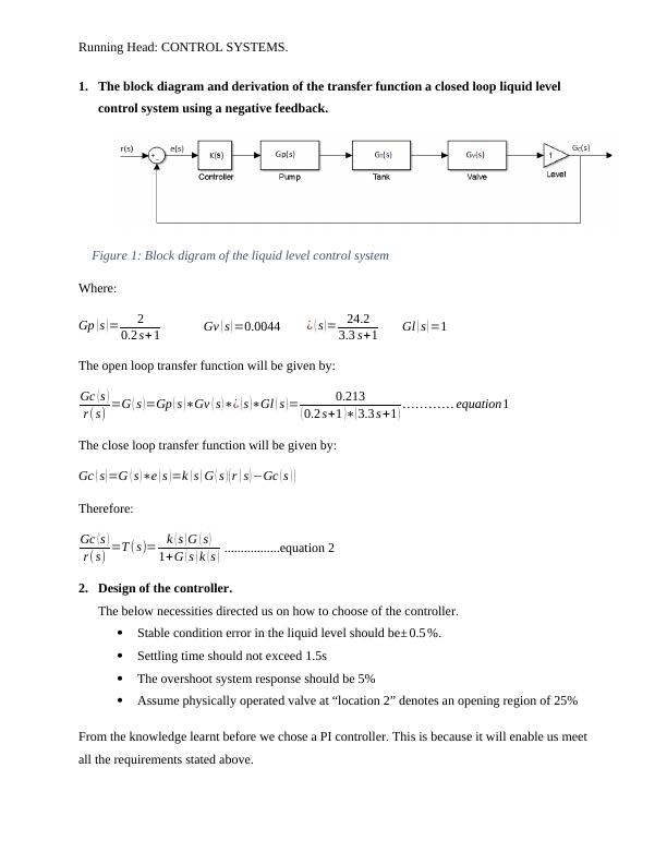
1. The block diagram and derivation of the transfer function a closed loop liquid level
control system using a negative feedback.
Figure 1: Block digram of the liquid level control system
Where:
Gp ( s ) = 2
0.2 s+ 1 Gv ( s ) =0.0044 ¿ ( s ) = 24.2
3.3 s+1 Gl ( s ) =1
The open loop transfer function will be given by:
Gc ( s )
r (s) =G ( s )=Gp ( s )∗Gv ( s )∗¿ ( s )∗Gl ( s )= 0.213
( 0.2 s+1 )∗( 3.3 s +1 ) ... ... ... ... equation1
The close loop transfer function will be given by:
Gc ( s )=G ( s )∗e ( s )=k ( s ) G ( s ) ( r ( s ) −Gc ( s ) )
Therefore:
Gc ( s )
r (s) =T (s)= k ( s ) G ( s )
1+G ( s ) k ( s ) .................equation 2
2. Design of the controller.
The below necessities directed us on how to choose of the controller.
Stable condition error in the liquid level should be± 0.5 %.
Settling time should not exceed 1.5s
The overshoot system response should be 5%
Assume physically operated valve at “location 2” denotes an opening region of 25%
From the knowledge learnt before we chose a PI controller. This is because it will enable us meet
all the requirements stated above.
Running Head: CONTROL SYSTEMS.
Design procedure for the controller.
kp ( s ) =kp + ki
s
Substituting for G(s) in equation 1
We have our closed loop transfer function as:
T ( s )=
k ( s )∗
[ 0.213
( 0.2 s+ 1 )∗( 3.3 s+1 ) ]
1+{k ( s )∗
[ 0.213
( 0.2 s+1 )∗( 3.3 s +1 ) ] .....................equation 3
Substituting for k ( s ) and solving the equation we have:
T ( s ) = 0.213 skp+ 0.213 ki
0.66 s3+ 3.5 s2+ s+ 0.213 skp +0.213 ki ........................equation 4
We obtained the value of Alpha (𝛼) in order to obtain Kp and Ki for a stable system as follows:
From equation 1 open loop transfer function, G(s) = 0.213
0.66 s2 +3.5 s +1
Finding the poles using the following quadratic equation:
−b ± √b2−4 ac
2 a
−3.5 ± √3.52−(4∗0.66∗1)
2∗0.66
Pole 1, P1 = −3.5+ √ 3.52−(4∗0.66∗1)
2∗0.66 = -0.3
Pole 2, P2 = −3.5− √3.52−(4∗0.66∗1)
2∗0.66 = -5
Alpha, 𝛼 < |P1+P2|
𝛼 < |-0.3+-5|
Running Head: CONTROL SYSTEMS.
𝛼 < 5.3
Value of 𝛼 chosen should not exceed summation of poles of the exposed loop system, the
system turns into a stable condition at all values of 𝐾𝑝 the value of alpha was selected to be 0.8.
The integral gain can be defined in terms of proportional gain as ki= K p (s+ α )
s .
The values of kp and ki were obtained by plotting the root locus and reading the gain values from
the plot:
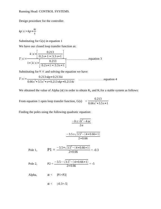
Matlab code:
Figure 2: code for calculating root locus
-10 -8 -6 -4 -2 0 2 4 6 8 10
-10
-8
-6
-4
-2
0
2
4
6
8
10
0.34
0.86
0.94
0.64
0.76
0.160.340.50.64
0.76
0.86
0.94
0.985
0.160.5
0.985
2
4
6
8
10
2
4
6
8
10
Root Locus
Real Axis (seconds-1)
Imaginary Axis (seconds-1)
System: Gmod
Gain: 30.5
Pole: -2.49 - 1.89i
Damping: 0.797
Overshoot (%): 1.59
Frequency (rad/s): 3.12
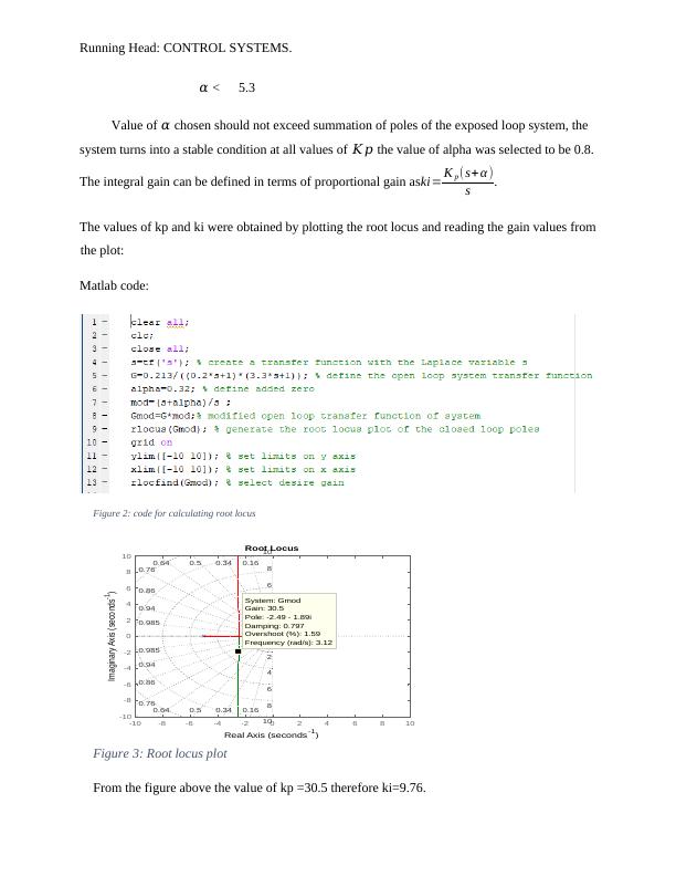
Figure 3: Root locus plot
From the figure above the value of kp =30.5 therefore ki=9.76.
𝛼 < 5.3
Value of 𝛼 chosen should not exceed summation of poles of the exposed loop system, the
system turns into a stable condition at all values of 𝐾𝑝 the value of alpha was selected to be 0.8.
The integral gain can be defined in terms of proportional gain as ki= K p (s+ α )
s .
The values of kp and ki were obtained by plotting the root locus and reading the gain values from
the plot:
Matlab code:
Figure 2: code for calculating root locus
-10 -8 -6 -4 -2 0 2 4 6 8 10
-10
-8
-6
-4
-2
0
2
4
6
8
10
0.34
0.86
0.94
0.64
0.76
0.160.340.50.64
0.76
0.86
0.94
0.985
0.160.5
0.985
2
4
6
8
10
2
4
6
8
10
Root Locus
Real Axis (seconds-1)
Imaginary Axis (seconds-1)
System: Gmod
Gain: 30.5
Pole: -2.49 - 1.89i
Damping: 0.797
Overshoot (%): 1.59
Frequency (rad/s): 3.12
Figure 3: Root locus plot
From the figure above the value of kp =30.5 therefore ki=9.76.
Running Head: CONTROL SYSTEMS.
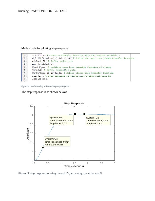
Matlab code for plotting step response.
Figure 4: matlab code for determining step response
The step response is as shown below:
0 0.5 1 1.5 2 2.5 3
0
0.2
0.4
0.6
0.8
1
1.2
Step Response
Time (seconds)
Amplitude
System: Gc
Time (seconds): 1.52
Amplitude: 1.02
System: Gc
Time (seconds): 1.87
Amplitude: 1.02
System: Gc
Time (seconds): 0.314
Amplitude: 0.286
Figure 5:step response settling time=1.7s,percentage overshoot=4%
End of preview
Want to access all the pages? Upload your documents or become a member.
Related Documents
Control and Instrumentation Doclg...
|53
|3958
|272
Control Design for F-18 Longitudinal Dynamicslg...
|6
|895
|81
Transient Response Improvement through Controller Designlg...
|2
|677
|500