Ask a question from expert
Coefficients Standardized - PDF
33 Pages4662 Words54 Views
Added on 2021-01-01
Coefficients Standardized - PDF
Added on 2021-01-01
BookmarkShareRelated Documents
HOMEWORK PROJECT 31Homework Project3

Table of Contents1.Title page...................................................................................12.Table of contents ...........................................................................23.Honesty statement..........................................................................34.Exercise4.6..........................................................................................................................35.Exercise4.12........................................................................................................................46.Exercise4.24........................................................................................................................57.Exercise4.32........................................................................................................................68.Exercise4.40........................................................................................................................79.Exercise6.6..........................................................................................................................810.Exercise10.6........................................................................................................................911.Exercise10.2......................................................................................................................1212.Exercise10.3......................................................................................................................1313.Appendices..........................................................................................................14

Honesty StatementI, Betsy Sophia Reed, promise that I did not reference or use any previous solutions or statisticsin this submission. I promise that all exercises are my original work and that no other individual,including a tutor, performed these statistics.

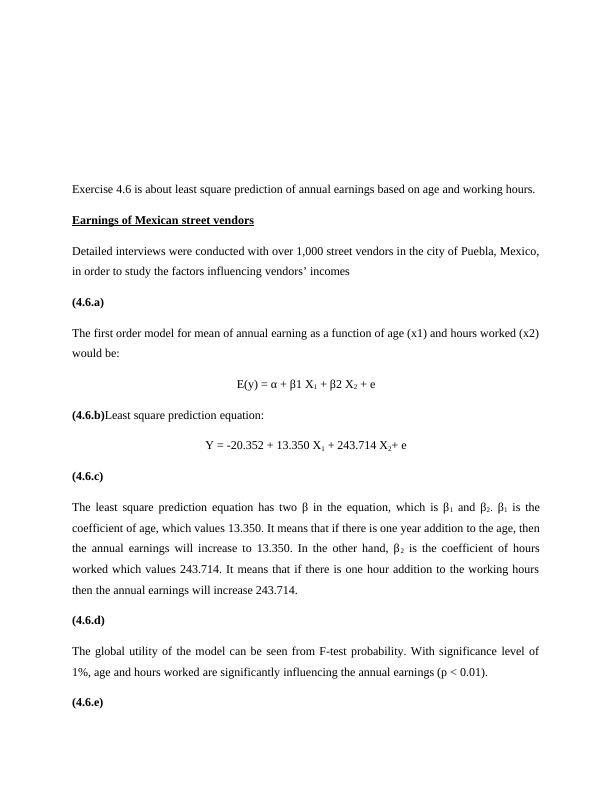
Exercise 4.6 is about least square prediction of annual earnings based on age and working hours.Earnings of Mexican street vendorsDetailed interviews were conducted with over 1,000 street vendors in the city of Puebla, Mexico,in order to study the factors influencing vendors’ incomes(4.6.a) The first order model for mean of annual earning as a function of age (x1) and hours worked (x2)would be:E(y) = α + β1 X1 + β2 X2 + e(4.6.b)Least square prediction equation:Y = -20.352 + 13.350 X1 + 243.714 X2+ e(4.6.c)The least square prediction equation has two β in the equation, which is β1 and β2. β1 is thecoefficient of age, which values 13.350. It means that if there is one year addition to the age, thenthe annual earnings will increase to 13.350. In the other hand, β2 is the coefficient of hoursworked which values 243.714. It means that if there is one hour addition to the working hoursthen the annual earnings will increase 243.714.(4.6.d)The global utility of the model can be seen from F-test probability. With significance level of1%, age and hours worked are significantly influencing the annual earnings (p < 0.01). (4.6.e)
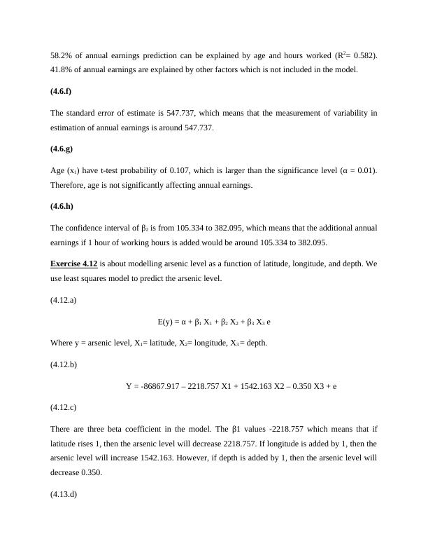
58.2% of annual earnings prediction can be explained by age and hours worked (R2= 0.582).41.8% of annual earnings are explained by other factors which is not included in the model.(4.6.f)The standard error of estimate is 547.737, which means that the measurement of variability inestimation of annual earnings is around 547.737.(4.6.g)Age (x1) have t-test probability of 0.107, which is larger than the significance level (α = 0.01).Therefore, age is not significantly affecting annual earnings.(4.6.h)The confidence interval of β2 is from 105.334 to 382.095, which means that the additional annualearnings if 1 hour of working hours is added would be around 105.334 to 382.095.Exercise 4.12 is about modelling arsenic level as a function of latitude, longitude, and depth. Weuse least squares model to predict the arsenic level.(4.12.a)E(y) = α + β1 X1 + β2 X2 + β3 X3 eWhere y = arsenic level, X1= latitude, X2= longitude, X3 = depth.(4.12.b)Y = -86867.917 – 2218.757 X1 + 1542.163 X2 – 0.350 X3 + e(4.12.c)There are three beta coefficient in the model. The β1 values -2218.757 which means that iflatitude rises 1, then the arsenic level will decrease 2218.757. If longitude is added by 1, then thearsenic level will increase 1542.163. However, if depth is added by 1, then the arsenic level willdecrease 0.350.(4.13.d)
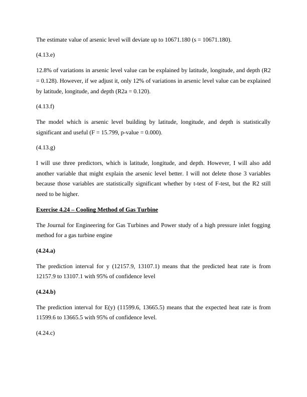
The estimate value of arsenic level will deviate up to 10671.180 (s = 10671.180).(4.13.e)12.8% of variations in arsenic level value can be explained by latitude, longitude, and depth (R2= 0.128). However, if we adjust it, only 12% of variations in arsenic level value can be explainedby latitude, longitude, and depth (R2a = 0.120).(4.13.f)The model which is arsenic level building by latitude, longitude, and depth is statisticallysignificant and useful (F = 15.799, p-value = 0.000).(4.13.g)I will use three predictors, which is latitude, longitude, and depth. However, I will also addanother variable that might explain the arsenic level better. I will not delete those 3 variablesbecause those variables are statistically significant whether by t-test of F-test, but the R2 stillneed to be higher.Exercise 4.24 – Cooling Method of Gas TurbineThe Journal for Engineering for Gas Turbines and Power study of a high pressure inlet foggingmethod for a gas turbine engine(4.24.a)The prediction interval for y (12157.9, 13107.1) means that the predicted heat rate is from12157.9 to 13107.1 with 95% of confidence level(4.24.b)The prediction interval for E(y) (11599.6, 13665.5) means that the expected heat rate is from11599.6 to 13665.5 with 95% of confidence level.(4.24.c)
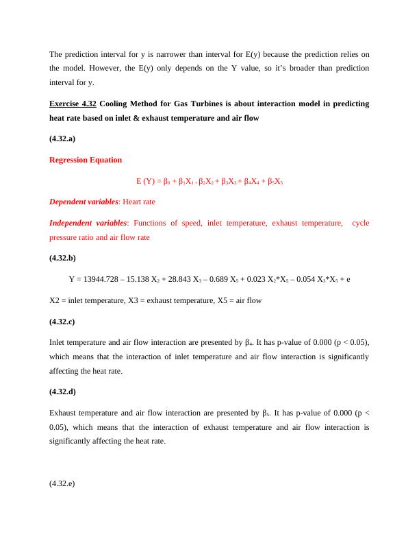
The prediction interval for y is narrower than interval for E(y) because the prediction relies onthe model. However, the E(y) only depends on the Y value, so it’s broader than predictioninterval for y.Exercise 4.32 Cooling Method for Gas Turbines is about interaction model in predictingheat rate based on inlet & exhaust temperature and air flow(4.32.a)Regression Equation E (Y) = β0 + β1X1 + β2X2 + β3X3 + β4X4 + β5X5Dependent variables: Heart rate Independent variables: Functions of speed, inlet temperature, exhaust temperature, cyclepressure ratio and air flow rate (4.32.b)Y = 13944.728 – 15.138 X2 + 28.843 X3 – 0.689 X5 + 0.023 X2*X5 – 0.054 X3*X5 + eX2 = inlet temperature, X3 = exhaust temperature, X5 = air flow(4.32.c)Inlet temperature and air flow interaction are presented by β4. It has p-value of 0.000 (p < 0.05),which means that the interaction of inlet temperature and air flow interaction is significantlyaffecting the heat rate.(4.32.d)Exhaust temperature and air flow interaction are presented by β5. It has p-value of 0.000 (p <0.05), which means that the interaction of exhaust temperature and air flow interaction issignificantly affecting the heat rate.(4.32.e)
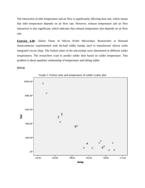
The interaction of inlet temperature and air flow is significantly affecting heat rate, which meansthat inlet temperature depends on air flow rate. However, exhaust temperature and air flowinteraction is also significant, which indicates that exhaust temperature also depends on air flowrate.Exercise 4.40– failure Times of Silicon Wafer Microchips. Researchers at NationalSemiconductor experimented with tin-lead solder bumps used to manufacture silicon waferintegrated circuit chips. The Failure times of the microchips were determined at different soldertemperatures. The researchers want to predict solder time based on solder temperature. Thisproblem is about quadratic relationship of temperature and failing solder(4.4.a)Graph 1. Failure time and temperature of solder scatter plot
End of preview
Want to access all the pages? Upload your documents or become a member.
Related Documents
Statistics for Financial Decisions Using Excellg...
|15
|3055
|88
OLS Regression Model for Estimating Unknown Coefficientslg...
|10
|2238
|406