CFD Simulation Report: Analysis of Fluid Flow in Rectangular Pipe

This report details a Computational Fluid Dynamics (CFD) analysis of fluid flow within a rectangular pipe, focusing on comparing inlet and outlet velocities and pressures. The methodology involves creating a 3D model, meshing, setting up boundary conditions in ANSYS Fluent, and running simulations. The analysis covers streamline, contour, and velocity vector flows, using the standard K-e viscous model. The report also discusses the advantages and disadvantages of CFD, such as cost and time savings versus accuracy limitations. Results include temperature variations in aluminum and copper square ducts under parallel and counter flow conditions. The simulation aims to provide a standard CFD simulation of a vehicle model and analyze the drag phenomenon between two cars.

CFD
[Document subtitle]
JANUARY 26, 2019
HP
[Company address]

Contents
General Information...........................................................................................................................................0
1. The objective of the simulation:- Main objective of CFD analysis is following.......................................0
Methodology......................................................................................................................................................0
Procedure............................................................................................................................................................9
Results..............................................................................................................................................................12
Advantage of CFD:..........................................................................................................................................15
Disadvantage of CFD:......................................................................................................................................15
Review..............................................................................................................................................................15
References........................................................................................................................................................16
II

General Information
1. The objective of the simulation:- Main objective of CFD analysis is following
a. Comparison of inlet and outlet velocity of fluid in Rectangular pipe.
b. Comparison of inlet and outlet presser of fluid in Rectangular pipe.
c. To show the streamline flow in Rectangular pipe in different position like fluid, solid, or
all domain.
d. To show the Contour flow in Rectangular pipe
e. To show the Velocity vector in Rectangular pipe
f. To produce a standard computational fluid dynamics simulation of a vehicle model and to
withdraw relevant data’s.
g. To produce standard of CFD simulations result of drag phenomenon to two cars that are
following eachother. (A., 1996)
Methodology
Step1. Make the 3d Module in the Cad software (Creo, Catia, Solid work, Unigraphix, or any
another cad software) according to given dimension then it convert into .IGS or .STP file.
Step 2. Start the workbench of the ansys software
Step3. Select the module
Example.
 Design as assessment
 Electric
 Explicit dynamic
 Fluid flow – blow molding (poly flow)
 Fluid flow – extrusion (poly flow)
 Fluid flow (CFX)

 Fluid flow (fluent)
 Fluid flow (poly flow)
 Harmonic response
 Hydrodynamic diffraction
 Hydrodynamic time response
 IC engine
 Linear Buckling
 Magnetostatic
 Modal
 Modal (samcef)
 Random vibration
 Response spectrum
 Rigid dynamics
 Static structural
 Static structural (samcef)
 Steady- state thermal
 Thermal electric
 Through flow
 Transient structural
 Transient thermal
Component systems
 Autodyne
 Blade gen
 CFX
 Engineering data
 Explicitly dynamic
 External connection
 External data
 Finite element modeller
 Fluent
1

 Fluent ( with T Grid meshing)
 Geometry
 ICEM CFD
 Icepak
 Mechanical APDL
 Mechanical Model
 Mesh
 Microsoft office excel
 Poly flow
 Poly flow – Blow Molding
 Poly flow – Extrusion
 Result
 System Coupling
 Turbo grid
 Vista AFD
 Vista CCD
 Vista CCD (with CCM)
 Vista CPD
 Vista RTD
 Vista TF
Custom systems
 FSI: Fluid Flow(CFX)
 FSI: Fluid Flow(Fluent)
 Pre Stress Modal
 Random Vibration
 Response Spectrum
 Thermal stress
Design Exploration
 Direct optimization
2

 Parameters correlation
 Response surface
 Response surface optimization
 Six sigma analysis
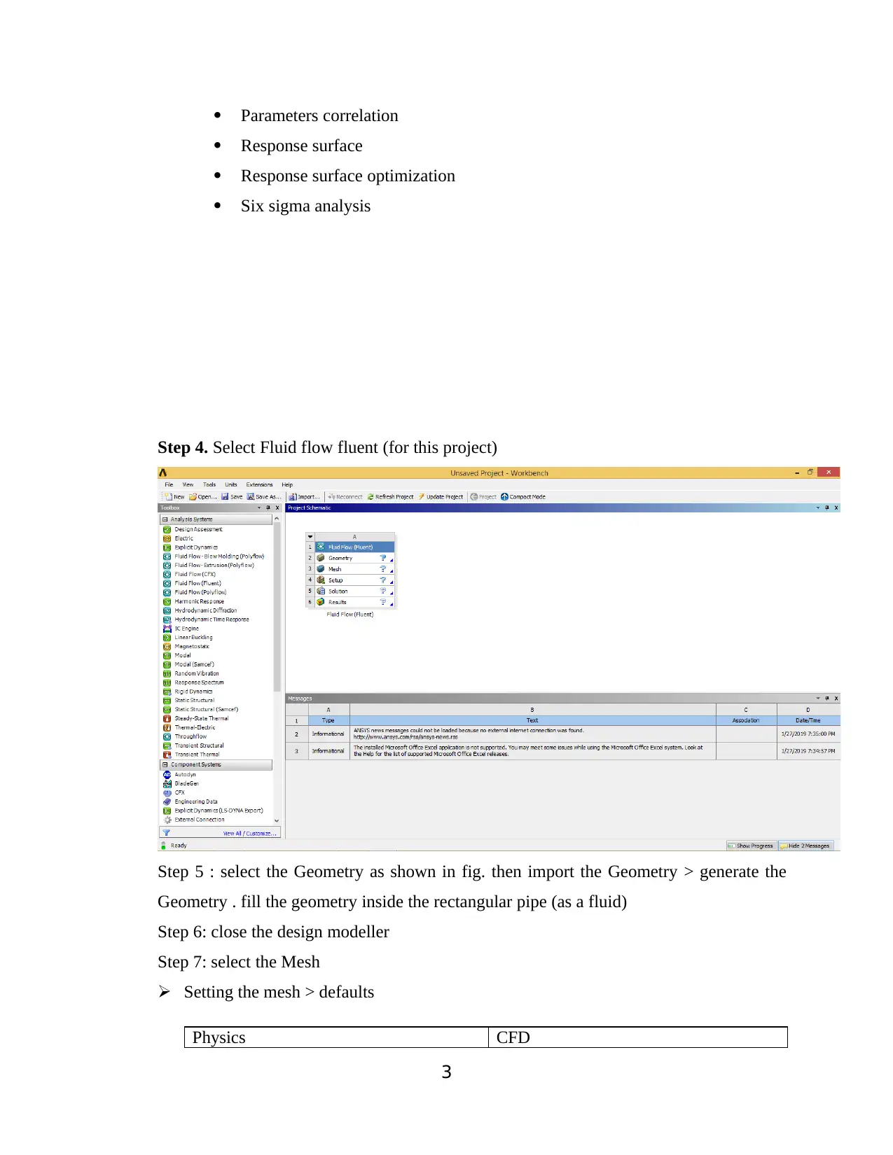
Step 4. Select Fluid flow fluent (for this project)
Step 5 : select the Geometry as shown in fig. then import the Geometry > generate the
Geometry . fill the geometry inside the rectangular pipe (as a fluid)
Step 6: close the design modeller
Step 7: select the Mesh
 Setting the mesh > defaults
Physics CFD
3

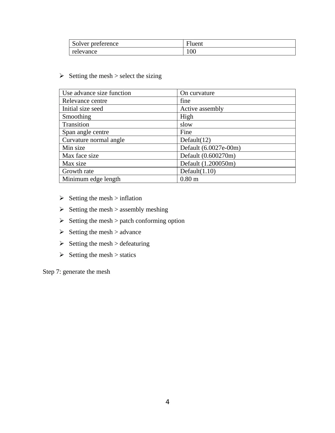
Solver preference Fluent
relevance 100
 Setting the mesh > select the sizing
Use advance size function On curvature
Relevance centre fine
Initial size seed Active assembly
Smoothing High
Transition slow
Span angle centre Fine
Curvature normal angle Default(12)
Min size Default (6.0027e-00m)
Max face size Default (0.600270m)
Max size Default (1.200050m)
Growth rate Default(1.10)
Minimum edge length 0.80 m
 Setting the mesh > inflation
 Setting the mesh > assembly meshing
 Setting the mesh > patch conforming option
 Setting the mesh > advance
 Setting the mesh > defeaturing
 Setting the mesh > statics
Step 7: generate the mesh
4

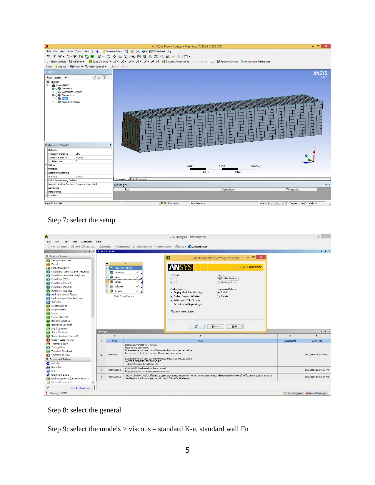
Step 7: select the setup
Step 8: select the general
Step 9: select the models > viscous – standard K-e, standard wall Fn
5

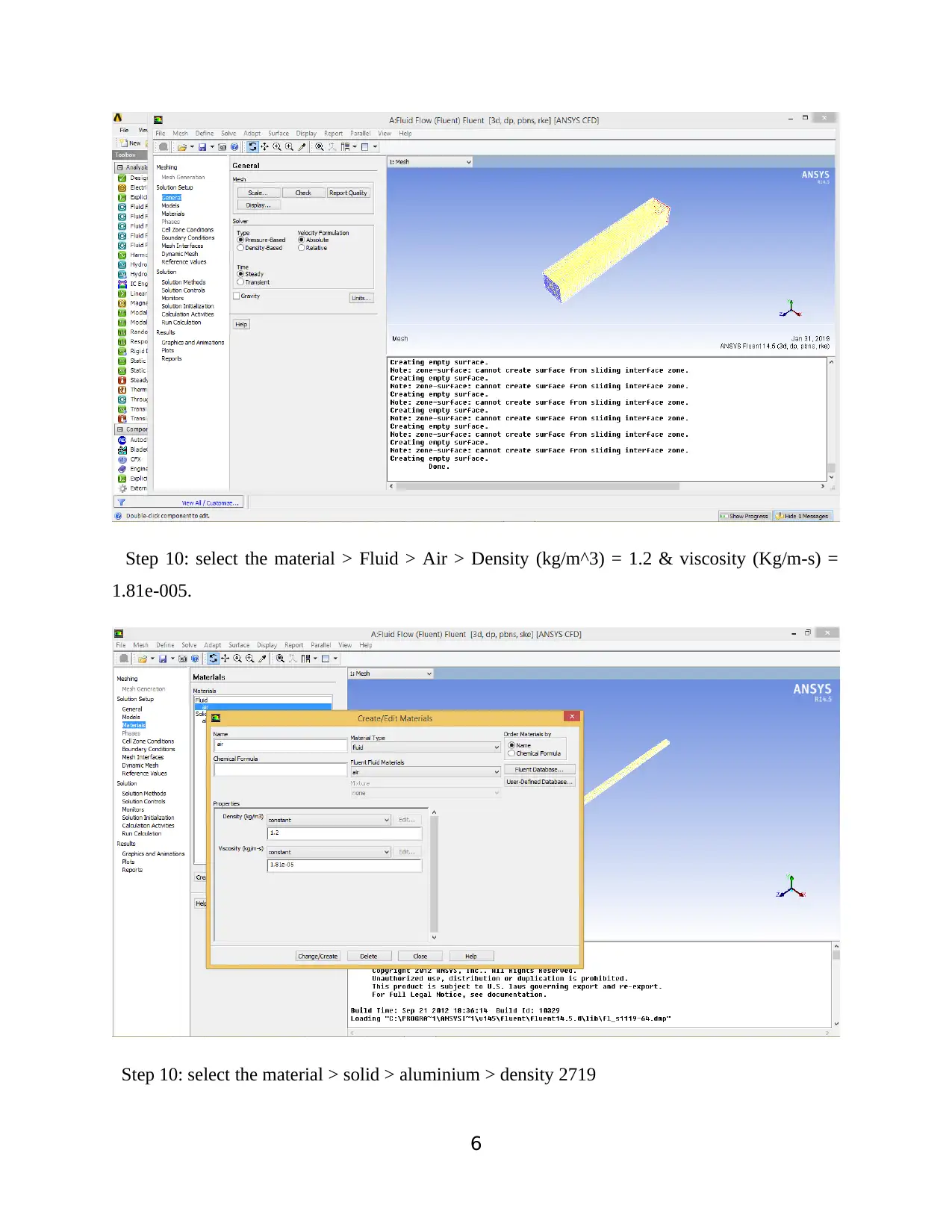
Step 10: select the material > Fluid > Air > Density (kg/m^3) = 1.2 & viscosity (Kg/m-s) =
1.81e-005.
Step 10: select the material > solid > aluminium > density 2719
6

Step 10: select the Boundary condition > inlet > edit > Velocity magnitude (m/s)
Step 10: select the Boundary condition > inlet > edit > turbulent intensity (%) =5 & turbulent
viscosity ratio = 10.
Step 11: select the Boundary condition > outlet > edit > gauge pressure (Pascal) =0, back flow
direction specification method > normal to Boundary , back flow turbulent intensity (%) = 5 &
back flow turbulent viscosity ratio = 10.
Step 12: select the solution > solution method > scheme > simple
Step 13: select the solution > solution method > spatial discretization > gradient > Least
Squares Cell Based
Step 14: select the solution > pressure > standard
Step 15: select the solution > momentum > second order upwind
Step 16: select the solution > Turbulent Kinetic energy > first order upwind
Step 17: select the solution > Turbulent dissipation rate > first order upwind
Step 18: select the control > pressure = 0.3 > density = 1 > body force = 1 > momentum = 0.7 >
turbulent Kinetic energy = 0.8.
Step 19: solution initialization > standard initialization > compute from inlet > reference frame
– relative to cell Zone > initial value > Gauge pressure = 0, X velocity (m/s) = 0, y velocity (m/s)
= 0, Z velocity (m/s) = -40, Turbulent Kinetic Energy (m2/s2) & turbulent dissipation rate (
m2/s3) = 21480.66
Step 20: run calculation > Number of Iterations = 60 > reporting interval = 1 > Profile update
Interval = 1.
Step 21: result > Graph and Animation
Step 22: result > plots
Step 23: result > reports
7

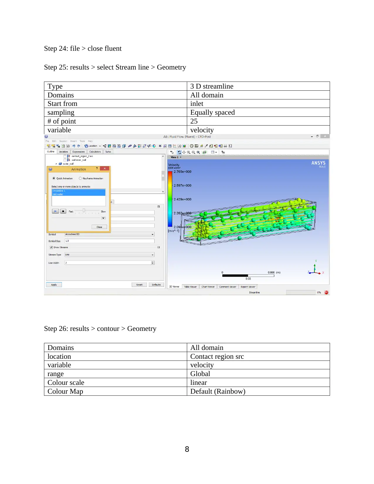
Step 24: file > close fluent
Step 25: results > select Stream line > Geometry
Type 3 D streamline
Domains All domain
Start from inlet
sampling Equally spaced
# of point 25
variable velocity
Step 26: results > contour > Geometry
Domains All domain
location Contact region src
variable velocity
range Global
Colour scale linear
Colour Map Default (Rainbow)
8

Procedure
1. Creation of vehicle model without an application of spoiler: - A vehicle model is
made by considering the given standards and construction points. The designed model is
of the defined computational domain using ANSYS software.
2. Creation of vehicle model with an application of spoiler: - The vehicle model
configuration is standardized by the length from front to rear of the car model.
3. Creation of 3D model in a given computational domain:- Some assumptions are
considered in order to develop the vehicle configuration from the given fabrication point
and then to subdue on to 3D air domain in the design model. The following presumption
is that the car must be forward moving with a constant velocity ‘V’ passing through the
air. Instead of the above presumption, it is interpreted that car is stationary, but the air is
moving with the same velocity in the opposite direction. The total computational domain
is done irrespective to the air domain. Therefore, the car is brought in the fluid domain,
with acceptable boundary conditions are allocated.
4. Meshing the model: - Meshing is the vital step for the simulation by ANSYS. Choosing
a acceptable mesh is the challenging task as a acceptable mesh will give relevent and
precise solution whereas mistaken meshing will provide imprecise solutions which will
make the analysis irrelevent. To examine the turbulence appropriately, entire mesh
should be grid all alone. Mesh must be as finer as fesible mainly at the boundary layer.
Apart from that, numerous mesh elements in the car model that conduct to finer meshing
will enlarge the computational cost therefore mesh size must be optimized in a controlled
manner. Precise and optimized computational cost will be obtained by making selection
proper mesh elements. Turbulence can be properly obtained when the mesh is done
independent and fine including boundary layers. The flow domains are split into smaller
subdomain. The sub domains are often called elements or cells and collections of these
cells called as the mesh. (Haecheon Choi, 2009)
9