Computational Fluid Dynamics: Simple Initial Value Problem and Numerical Method for Predicting Vibration of Cylinder

Computational Fluid Dynamics 1
COMPUTATIONAL FLUID DYNAMICS
By Name
Course
Professor
University
City/State
Date

Computational Fluid Dynamics 2
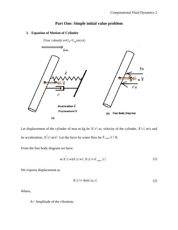
Part One: Simple initial value problem
1. Equation of Motion of Cylinder
Let displacement of the cylinder of mas m kg be X (t) m, velocity of the cylinder, ̇X (t) m/s and
its acceleration, ̈X (t) m/s2. Let the force by water flow be Fwater (t ) N.
From the free body diagram we have:
m ̈X ( t ) + kX (t)+C ̇X (t)=Fwater (t) (1)
We express displacement as
X (t)= Asin(ω1 t) (2)
Where,
A= Amplitude of the vibration;

Computational Fluid Dynamics 3
ω1= Angular velocity of the vibration, rad/s.
We therefore have velocity as:
̇X (t)= A ω1 cos (ω1 t) (3)
And Acceleration as:
̈X (t)=− A ω1
2 sin (ω1 t) (4)
̈X (t)=−ω1
2 X (t) (5)
Force, Fwater, on the cylinder is expressed as:
Fwater ( t )=CA md
d V r
dt + ρC D A p
2 |V r|V r (6)
Where,
CD=Coefficient of drag;
C A=Coefficient of inertia;
Ap= Surface area of the cylinder experiencing drag, m2;
|V r|= Magnitude of vibration velocity;
V r=Velocity of flow relative to cylinder, m/s; same as u- ̇X (t);
md=Displacement fluid mass, kg;
ρ= Density of water, kgm-3;
u= Flow velocity, m/s.

Computational Fluid Dynamics 4
Using Equation 6 we have:-
Fwater ( t ) =CA md
d V r
dt + ρC D A p
2 |V r|V r (7)
u=U0 +Um sin ( ωt )
V r =u− ̇X (t)
V r =U0 +Um sin ( ωt )− A ω1 cos(ω1 t)
d V r
dt =Um ωcos ( ωt ) + A ω1
2 sin(ω1 t )
Fwater ( t ) =CA md U m ωcos ( ωt ) +C A md A ω1
2 sin(ω1 t )+ ρC D Ap
2 |V r|( U 0+ Um sin ( ωt ) − A ω1 cos (ω1 t) )
(8)
Equation of motion becomes:
m ̈X ( t ) + kX (t)+C ̇X (t)=C A md Um ωcos ( ωt ) ¿+C A md A ω1
2 sin(ω1 t)+ ρC D A p
2 |V r|( U0 +U m sin ( ωt ) −A ω1 cos
Which becomes:
( m+C A md ) ̈X ( t ) + ( C + ρCD A p
2 |V r|) ̇X +kX ( t ) =C A md Um ωcos ( ωt ) ¿+ ρC D A p
2 |V r|( U0 +Um sin ( ωt ) )
(9)
We will use Euler – Runge Kutta method.
Runge Kutta method is of the form
dy
dx =f ( x , y ) , y ( 0 ) , y0 (10)

Computational Fluid Dynamics 5
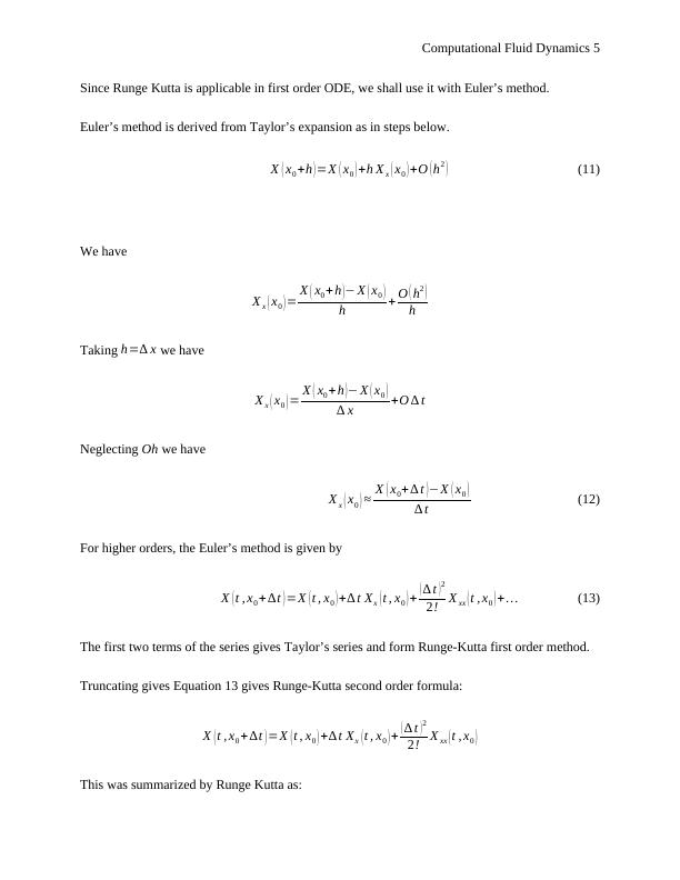
Since Runge Kutta is applicable in first order ODE, we shall use it with Euler’s method.
Euler’s method is derived from Taylor’s expansion as in steps below.
X ( x0 +h ) =X ( x0 ) +h X x ( x0 ) +O ( h2 ) (11)
We have
X x ( x0 ) = X ( x0 + h )− X ( x0 )
h + O ( h2 )
h
Taking h=∆ x we have
X x ( x0 ) = X ( x0 + h )− X ( x0 )
∆ x +O ∆ t
Neglecting Oh we have
X x ( x0 ) ≈ X ( x0+ ∆ t )−X ( x0 )
∆ t (12)
For higher orders, the Euler’s method is given by
X ( t , x0 + ∆t ) =X ( t , x0 ) +∆ t Xx ( t , x0 ) + ( ∆ t ) 2
2! X xx ( t , x0 ) + ... (13)
The first two terms of the series gives Taylor’s series and form Runge-Kutta first order method.
Truncating gives Equation 13 gives Runge-Kutta second order formula:
X ( t , x0 + ∆t ) =X ( t , x0 ) +∆ t Xx ( t , x0 ) + ( ∆ t ) 2
2! X xx ( t , x0 )
This was summarized by Runge Kutta as:

Computational Fluid Dynamics 6
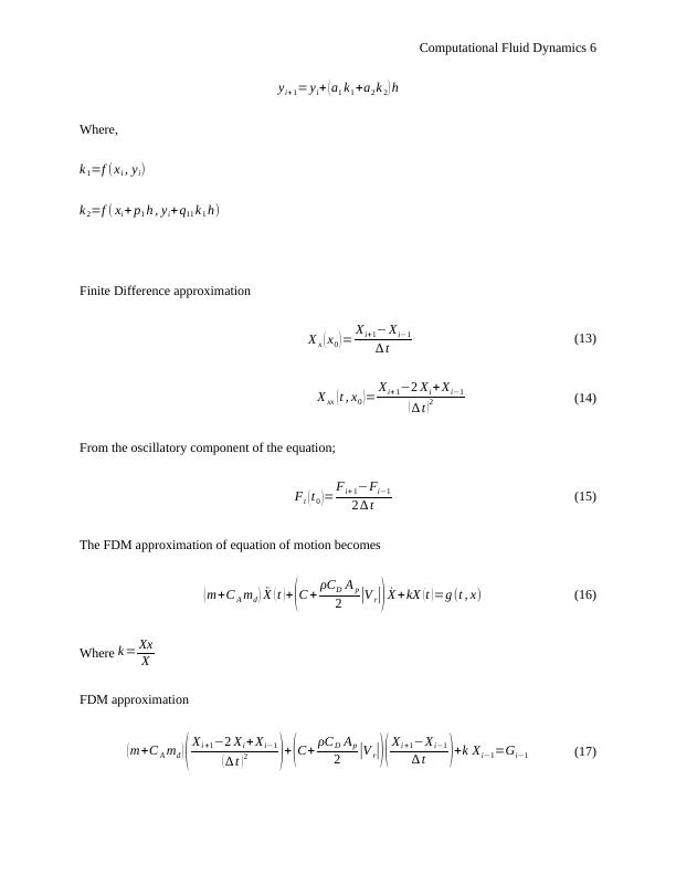
yi+ 1= yi+ ( a1 k1 +a2 k 2 ) h
Where,
k 1=f (xi , yi)
k 2=f ( xi + p1 h , yi+ q11 k1 h)
Finite Difference approximation
X x ( x0 ) = Xi+1− Xi−1
∆ t (13)
X xx ( t , x0 )= Xi+ 1−2 Xi + Xi−1
( ∆ t ) 2 (14)
From the oscillatory component of the equation;
Ft ( t0 )= Fi+ 1−Fi−1
2 ∆ t (15)
The FDM approximation of equation of motion becomes
( m+C A md ) ̈X ( t )+ (C + ρCD A p
2 |V r|) ̇X + kX (t )=g (t , x) (16)
Where k = Xx
X
FDM approximation
( m+C A md ) ( Xi +1−2 Xi + Xi−1
( ∆ t )2 )+ (C+ ρC D Ap
2 |V r|)( Xi +1−Xi−1
∆ t )+k Xi−1=Gi−1 (17)

Computational Fluid Dynamics 7
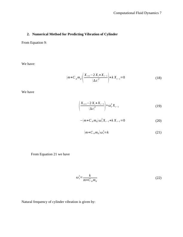
2. Numerical Method for Predicting Vibration of Cylinder
From Equation 9:
We have:
( m+C A md ) ( Xi +1−2 Xi + Xi−1
( ∆ t )2 )+ k Xi−1=0 (18)
We have
( Xi +1−2 Xi + Xi−1
( ∆ t )
2 ) ≈ ω1
2 Xi−1 (19)
− ( m+C A md ) ω1
2 Xi−1 +k X i−1 =0 (20)
( m+C A md ) ω1
2=k (21)
From Equation 21 we have
ω1
2= k
m+C A md
(22)
Natural frequency of cylinder vibration is given by:

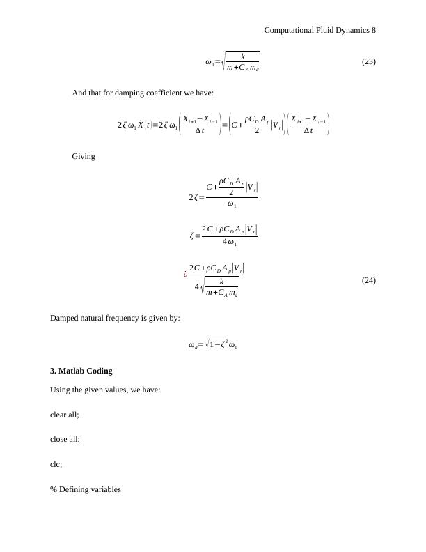
Computational Fluid Dynamics 8
ω1= √ k
m+C A md
(23)
And that for damping coefficient we have:
2 ζ ω1 ̇X ( t )=2 ζ ω1 ( Xi +1−Xi−1
∆ t )= (C + ρCD A p
2 |V r|)( X i+1−X i−1
∆ t )
Giving
2 ζ=
C + ρC D A p
2 |V r|
ω1
ζ =2 C + ρC D A p |V r|
4 ω1
¿ 2C + ρC D A p |V r|
4 √ k
m+CA md
(24)
Damped natural frequency is given by:
ωd= √1−ζ2 ω1
3. Matlab Coding
Using the given values, we have:
clear all;
close all;
clc;
% Defining variables