Constraint : Monotone or Anti-monotone Convertible
VerifiedAdded on 2022/08/24
|10
|1582
|23
AI Summary
Contribute Materials
Your contribution can guide someone’s learning journey. Share your
documents today.
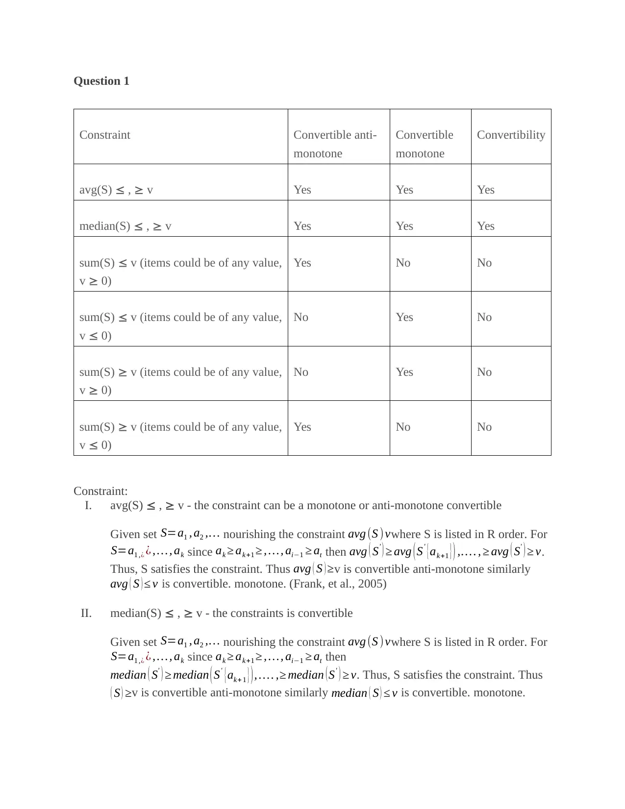
Question 1
Constraint Convertible anti-
monotone
Convertible
monotone
Convertibility
avg(S) , v Yes Yes Yes
median(S) , v Yes Yes Yes
sum(S) v (items could be of any value,
v 0)
Yes No No
sum(S) v (items could be of any value,
v 0)
No Yes No
sum(S) v (items could be of any value,
v 0)
No Yes No
sum(S) v (items could be of any value,
v 0)
Yes No No
Constraint:
I. avg(S) , v - the constraint can be a monotone or anti-monotone convertible
Given set S=a1 , a2 ,… nourishing the constraint avg (S ) vwhere S is listed in R order. For
S=a1 ,¿ ¿ , … , ak since ak ≥ ak+1 ≥ , …, ai−1 ≥ at then avg ( S' ) ≥ avg ( S' { ak+1 } ) ,… . , ≥ avg ( S' ) ≥ v.
Thus, S satisfies the constraint. Thus avg ( S ) ≥v is convertible anti-monotone similarly
avg ( S ) ≤ v is convertible. monotone. (Frank, et al., 2005)
II. median(S) , v - the constraints is convertible
Given set S=a1 , a2 ,… nourishing the constraint avg (S ) vwhere S is listed in R order. For
S=a1 ,¿ ¿ , … , ak since ak ≥ ak+1 ≥ , …, ai−1 ≥ at then
median ( S' ) ≥ median ( S' {ak+ 1 } ) , … . ,≥ median ( S' ) ≥ v. Thus, S satisfies the constraint. Thus
( S ) ≥v is convertible anti-monotone similarly median ( S ) ≤ v is convertible. monotone.
Secure Best Marks with AI Grader
Need help grading? Try our AI Grader for instant feedback on your assignments.
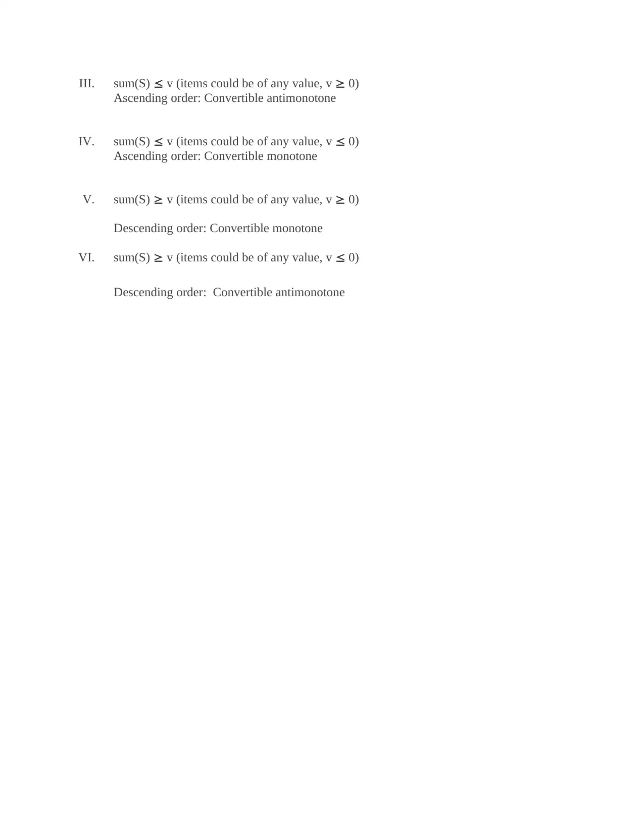
III. sum(S) v (items could be of any value, v 0)
Ascending order: Convertible antimonotone
IV. sum(S) v (items could be of any value, v 0)
Ascending order: Convertible monotone
V. sum(S) v (items could be of any value, v 0)
Descending order: Convertible monotone
VI. sum(S) v (items could be of any value, v 0)
Descending order: Convertible antimonotone
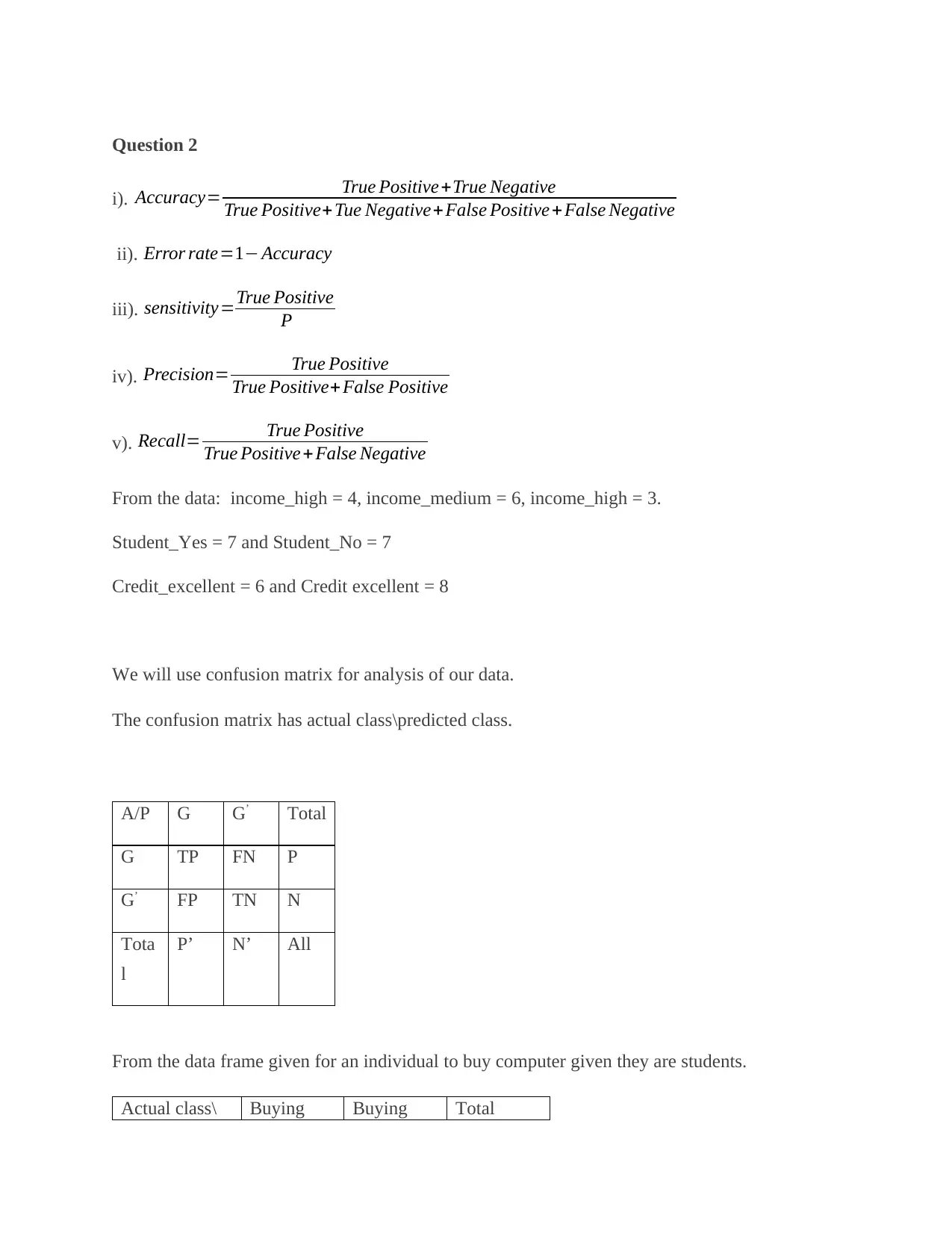
Question 2
i). Accuracy= True Positive +True Negative
True Positive+Tue Negative+ False Positive +False Negative
ii). Error rate=1− Accuracy
iii). sensitivity=True Positive
P
iv). Precision= True Positive
True Positive+ False Positive
v). Recall= True Positive
True Positive + False Negative
From the data: income_high = 4, income_medium = 6, income_high = 3.
Student_Yes = 7 and Student_No = 7
Credit_excellent = 6 and Credit excellent = 8
We will use confusion matrix for analysis of our data.
The confusion matrix has actual class\predicted class.
A/P G G’ Total
G TP FN P
G’ FP TN N
Tota
l
P’ N’ All
From the data frame given for an individual to buy computer given they are students.
Actual class\ Buying Buying Total
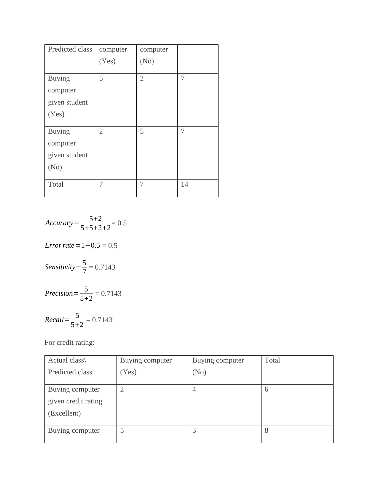
Predicted class computer
(Yes)
computer
(No)
Buying
computer
given student
(Yes)
5 2 7
Buying
computer
given student
(No)
2 5 7
Total 7 7 14
Accuracy= 5+2
5+5+2+2 = 0.5
Error rate=1−0.5 = 0.5
Sensitivity= 5
7 = 0.7143
Precision= 5
5+2 = 0.7143
Recall= 5
5+2 = 0.7143
For credit rating:
Actual class\
Predicted class
Buying computer
(Yes)
Buying computer
(No)
Total
Buying computer
given credit rating
(Excellent)
2 4 6
Buying computer 5 3 8
(Yes)
computer
(No)
Buying
computer
given student
(Yes)
5 2 7
Buying
computer
given student
(No)
2 5 7
Total 7 7 14
Accuracy= 5+2
5+5+2+2 = 0.5
Error rate=1−0.5 = 0.5
Sensitivity= 5
7 = 0.7143
Precision= 5
5+2 = 0.7143
Recall= 5
5+2 = 0.7143
For credit rating:
Actual class\
Predicted class
Buying computer
(Yes)
Buying computer
(No)
Total
Buying computer
given credit rating
(Excellent)
2 4 6
Buying computer 5 3 8
Secure Best Marks with AI Grader
Need help grading? Try our AI Grader for instant feedback on your assignments.
given credit rating
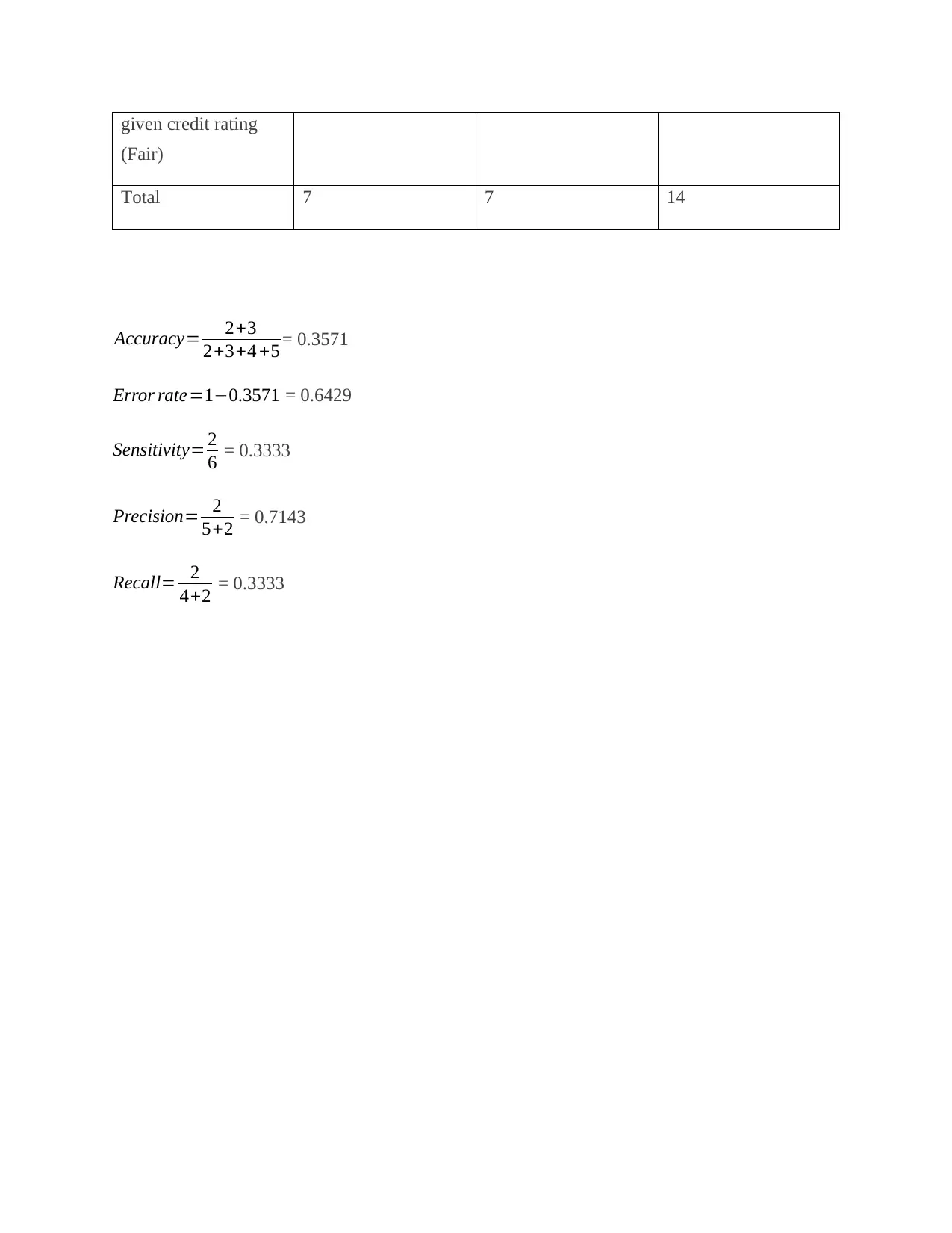
(Fair)
Total 7 7 14
Accuracy= 2+3
2+3+4 +5 = 0.3571
Error rate=1−0.3571 = 0.6429
Sensitivity= 2
6 = 0.3333
Precision= 2
5+2 = 0.7143
Recall= 2
4+2 = 0.3333
(Fair)
Total 7 7 14
Accuracy= 2+3
2+3+4 +5 = 0.3571
Error rate=1−0.3571 = 0.6429
Sensitivity= 2
6 = 0.3333
Precision= 2
5+2 = 0.7143
Recall= 2
4+2 = 0.3333
Question 3
Semi-Supervised Classification
Is one of the classification techniques that has brought attention in the field ranging from web
mining to bioinformatic since it is easy to obtain labeled and unlabeled data given it requires less
effort, time consumption and expertise. It aims at improving supervised classification through
minimizing errors in labeled data and should be compatible with distribution of unlabeled data.
The classification of algorithm mostly depends on conjectures they make on the relation between
unlabeled and labeled data disseminations. They are based on cluster assumption and manifold
assumption (S. Garcia, et al, 2014).
Semi-supervised classification can be divided into transductive and inductive learning. Where
transductive learning involves prediction of the labels of unlabeled data when prior knowledge if
given, takes tagged data and untagged data together to train the hypothesis that was used to label
the data sets. While inductive learning contemplates the provided tagged data and uncategorized
data as the training dataset, and then predict unobserved data.
Precision of text classifiers is enhanced through enhancing a minor quantity of tagged training
data with many unlabeled documents. This is significant because it is expensive to attain training
tags in most of text classification problems. Hence, in semi-supervised classification use of
unlabeled data help to reduce the classification error (Isaac Trigueroa, et al., 2013).
Comparing the semi-supervised classification methods semi-supervised Bayesian ARTMAP
achieves a good performance compared to Bayesian ARTMAP and the expectation
maximization algorithm. Hence, semi-supervised Bayesian ARTMAP is the most preferred
algorithm to perform semi-supervised classification task given it works with large amount of
unlabeled data sets and its demand on classification accuracy (Don Mitchell Wilkes, et al., 2020).
Why use semi-supervised learning:
This is the intermediate between supervised and unsupervised learning and uses both tagged and
untagged data in model fitting. The algorithm is trained upon combination of categorized and
uncategorized data.
When there is lack of enough labeled data to an accurate model and it is hard to resource data,
use semi-supervised learning can be used to increase the size of the training dataset. This helps to
stun the problematic of supervised learning since the quantity of tagged data is often smaller than
the untagged/partially categorized data samples also the unlabeled data is always cheap (I
Goodfellow, et al., 2016).
The algorithm uses three assumptions that is continuity assumption, clustering assumptions and
manifold. These assumptions make it easy to train unlabeled data set using classified labeled
data.
Semi-supervised learning is widely applied in many industries starting from fintech up to
entertainment industries. This algorithm can be used in speech analysis since labelling of audio
files is a very difficult task. The algorithm is important in internet content classification given
labelling of the webpages is unfeasible and impractical process. Also google search algorithm
depends on semi-supervised algorithm in ranking the relevance of every webpage for given
query. The algorithm is also widely used in protein sequence classification since DNA strands
are large sized. In banking the algorithm is used by banks to develop data security since the
developer knows few cases of cybercrimes. Given the developer does not know about the
remaining cases but he has to detect all the instances, the machine will have to find the rest of the
cases to prevent future frauds (Anastacia, 2013).
Paraphrase This Document
Need a fresh take? Get an instant paraphrase of this document with our AI Paraphraser
Question 4
Data clustering is a system of unsupervised classification given the clusters are formed by
estimating similarity and dissimilarity of basic characteristics between different cases of
variables. K-means is used for clustering technique when assembling large datasets.
There are three most used K-means clustering algorithm which are the MacQueen algorithm,
Hartigan and Won algorithm and the Forgy/Lloyd algorithm. The choice to use any of the
algorithm depends on size of the data, number of variables in the cases and how many clusters
are present in the data.
Let the set of data points be Y = {y1, y2, y3,..,yn} and W = {w1,w2,…….,wc} be the set of centers.
Step 1: Initialization
Specify the number of clusters by randomly choosing K data point from dataset as the initial
center of the clusters since the center is not yet known.
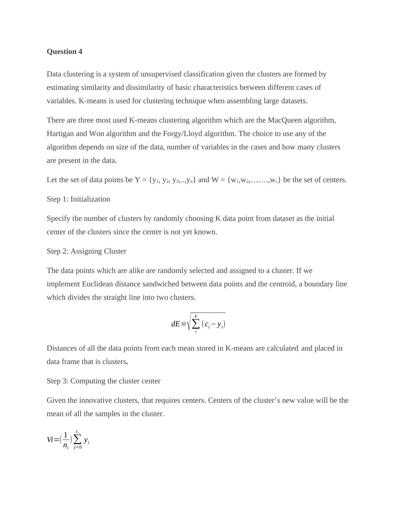
Step 2: Assigning Cluster
The data points which are alike are randomly selected and assigned to a cluster. If we
implement Euclidean distance sandwiched between data points and the centroid, a boundary line
which divides the straight line into two clusters.
dE= √ ∑
i
k
( ci − yi)
Distances of all the data points from each mean stored in K-means are calculated and placed in
data frame that is clusters.
Step 3: Computing the cluster center
Given the innovative clusters, that requires centers. Centers of the cluster’s new value will be the
mean of all the samples in the cluster.
Vi=( 1
ni
)∑
j=0
ci
yi
Data clustering is a system of unsupervised classification given the clusters are formed by
estimating similarity and dissimilarity of basic characteristics between different cases of
variables. K-means is used for clustering technique when assembling large datasets.
There are three most used K-means clustering algorithm which are the MacQueen algorithm,
Hartigan and Won algorithm and the Forgy/Lloyd algorithm. The choice to use any of the
algorithm depends on size of the data, number of variables in the cases and how many clusters
are present in the data.
Let the set of data points be Y = {y1, y2, y3,..,yn} and W = {w1,w2,…….,wc} be the set of centers.
Step 1: Initialization
Specify the number of clusters by randomly choosing K data point from dataset as the initial
center of the clusters since the center is not yet known.
Step 2: Assigning Cluster
The data points which are alike are randomly selected and assigned to a cluster. If we
implement Euclidean distance sandwiched between data points and the centroid, a boundary line
which divides the straight line into two clusters.
dE= √ ∑
i
k
( ci − yi)
Distances of all the data points from each mean stored in K-means are calculated and placed in
data frame that is clusters.
Step 3: Computing the cluster center
Given the innovative clusters, that requires centers. Centers of the cluster’s new value will be the
mean of all the samples in the cluster.
Vi=( 1
ni
)∑
j=0
ci
yi
Where ni is the quantity of data points in the ith cluster.
Step 2 and 3 are iterated until the K-means algorithm is converged.
Step 4: Convergence Condition
This process stops when the iterations number given of is attained. This process should stop
when there is no altering of data objects among the groups and when a threshold value is
obtained. If the circumstances are not satisfied, then repeat step 2and 3 again and complete the
whole process till the current settings will not be satisfied.
REFERENCE
1. S. García, Triguero and F. Herrera (2014): Self-Labeled Techniques for Semi-Supervised
Learning: Taxonomy, Software and Empirical Study.
2. Anastacia, 2013: Semi-Supervised Machine Learning Algorithms
3. I. H., & Frank, E. (2005). Data mining: Practical machine learning tools and techniques,
2nd edition. Morgan Kaufmann, San Francisco.
4. Isaac Trigueroa, José A. Sáeza, Julián Luengob, Salvador Garcíac, Francisco Herreraa,
2013: On the characterization of noise filters for self-training semi-supervised in nearest
neighbor classification.
5. I Goodfellow, Y Bengio, A Courville – 2016: Deep learning.
6. Xiaochun Wang, Xiali Wang, Don Mitchell Wilkes. 2020. Supervised Learning for Data
Classification Based Object Recognition
1 out of 10
Your All-in-One AI-Powered Toolkit for Academic Success.
+13062052269
info@desklib.com
Available 24*7 on WhatsApp / Email
![[object Object]](/_next/static/media/star-bottom.7253800d.svg)
Unlock your academic potential
© 2024 | Zucol Services PVT LTD | All rights reserved.