Business Statistics Analysis Report with Sample Data and Analysis

This report provides a detailed analysis of business statistics with sample data. It covers four different parts, including unique dataset, scatter plot, confidence interval, and summary of data. The report is useful for managers and business owners to make better decisions and planning.

Contents
REPORT ON BUSINESS STATISTICS ANALYSIS...............................................................................................1
Executive summary.....................................................................................................................................1
Introduction.................................................................................................................................................1
Part 1.......................................................................................................................................................2
Part 2.......................................................................................................................................................5
Part 3.......................................................................................................................................................7
Part 4.......................................................................................................................................................7
References...................................................................................................................................................8
REPORT ON BUSINESS STATISTICS ANALYSIS
Executive summary
When most managers want to recruit new staffs or employees, it’s better for them carry out
statistics analysis on the business. This helps them in better decision making and good planning.
Therefore most of these statistics analysis have been discussed in the sample report which
comprises of four different parts namely part 1, part 2, part 3 and part 4.
Introduction
Each and every business needs to maximize profit and minimize cost. This can only be achieved
through analysis of the data by a data analyst and later use the result from the analysis to advice
the manager or business owner.

Part 1
The unique dataset consist of six variables and 200 observations. The variables are the unique
student id number, the sample, the region, payment for version 1, amount of payment for version
1 and the amount of payment for version 2. The average of the variable how much would they
pay for version 1 is 1003.30 for region A and for region B of the same variable is 1039.59. The
standard deviation of the variable how much would they pay is 105.88 for region A and 125.80
for region B. The number of observations for the variable how much would they pay for version
1 is 104 for A and 96 for region B. Therefore we observe that both the mean and standard
deviation for the variable how much would they pay for version 1 is higher in region B than that
of region A. However the count of the variable how much would they pay for version 1 is greater
in region A than that of region B. This higher number of count of this attribute in region A
contributes to the mean and standard deviation for region A to be lesser than that of region B.
Therefore the higher the population/count, the smaller the mean or standard deviation of the
given variable. Again using the scatter plot we can see the relationship between the variables
how much would they pay for version 1 and how much would they pay for version 2. We
visualize that since the R-square of these two variables are 0.98 or 98% which means that the
variable how much would they pay for version 2 (dependent variable) is predicted by the
independent variable (how much would they pay for version 1). Furthermore, it also means that
98% of the variable how much would they pay for version 2 is predicted by the independent
variable. The R-square is positive and is almost approaching 1 and therefore it perfectly show
that the variable how much would they pay for version 1 and that of version 2 are well related
and therefore need to be maintained. From the scatter plot we can also observe that as the
variable how much would they pay for version 1 increase with a decrease in the variable how
much would they pay for version 2. Now on using the variable which region and would they pay

more for version1. We realize that the count of the variable would they pay more for version 1
for region A is 45 for no and 59 for yes. For region B the count of this variable is 33 for no and
59 for yes. The total count of the variable would they pay more for version 1 is 78 for no and 122
for yes. From these two variables we can see that the count of variable would they pay more for
version 1 for yes is always higher than that of no for region A and B. Again we notice that the
count of variable would they pay more for version 1 for no is higher in region A than region B
however the count of the variable would they pay more for version 1 for yes is greater in region
B than region A. The total count of the attribute would they pay more for version 1 for region A
including both yes and no are 104 and that for B is 96. I would recommend that the count of
would they pay more for version 1 for region B for no should be increased and that for yes to be
decreased so that they do not have a large difference between them, but I would recommend that
the count of would they pay more for version 1 for region A to be maintained for both yes and no
because the difference between them is minimal. The % count of the variable would they pay
more for version 1 for region A is 43.27% for no and 56.73% for yes. Additionally, the % count
of the variable would they pay more for version 1 for region B is 34.38% for no and 65.63% for
yes. The total % count of this variable for both region A and B is 39% for no and 61% for yes.
Also the % count of this variable for region A is higher than that of B for no and for yes it’s the
vice versa (Cameron, 2009). The number of people who would pay more for version 1 is 2772
for no and those for yes are 4128. The total for both yes and no for those who would pay more
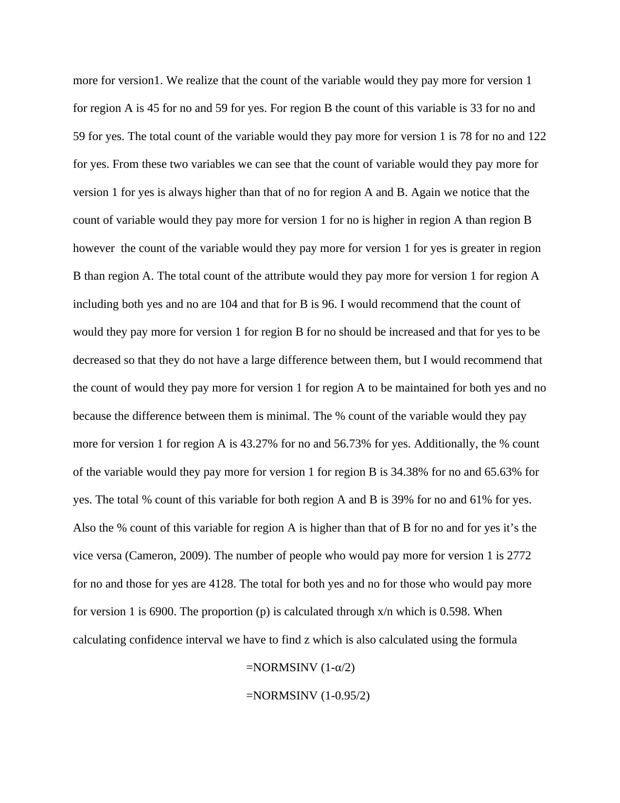
for version 1 is 6900. The proportion (p) is calculated through x/n which is 0.598. When
calculating confidence interval we have to find z which is also calculated using the formula
=NORMSINV (1-α/2)
=NORMSINV (1-0.95/2)

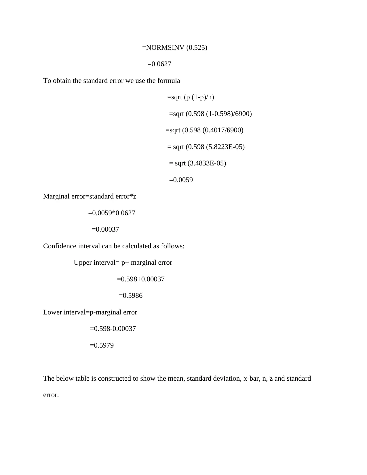
=NORMSINV (0.525)
=0.0627
To obtain the standard error we use the formula
=sqrt (p (1-p)/n)
=sqrt (0.598 (1-0.598)/6900)
=sqrt (0.598 (0.4017/6900)
= sqrt (0.598 (5.8223E-05)
= sqrt (3.4833E-05)
=0.0059
Marginal error=standard error*z
=0.0059*0.0627
=0.00037
Confidence interval can be calculated as follows:
Upper interval= p+ marginal error
=0.598+0.00037
=0.5986
Lower interval=p-marginal error
=0.598-0.00037
=0.5979
The below table is constructed to show the mean, standard deviation, x-bar, n, z and standard
error.

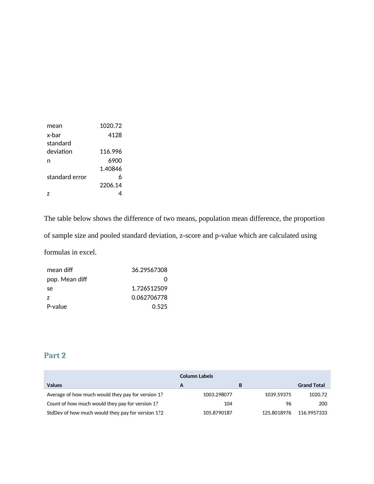
mean 1020.72
x-bar 4128
standard
deviation 116.996
n 6900
standard error
1.40846
6
z
2206.14
4
The table below shows the difference of two means, population mean difference, the proportion
of sample size and pooled standard deviation, z-score and p-value which are calculated using
formulas in excel.
mean diff 36.29567308
pop. Mean diff 0
se 1.726512509
z 0.062706778
P-value 0.525
Part 2
Column Labels
Values A B Grand Total
Average of how much would they pay for version 1? 1003.298077 1039.59375 1020.72
Count of how much would they pay for version 1? 104 96 200
StdDev of how much would they pay for version 1?2 105.8790187 125.8018976 116.9957333

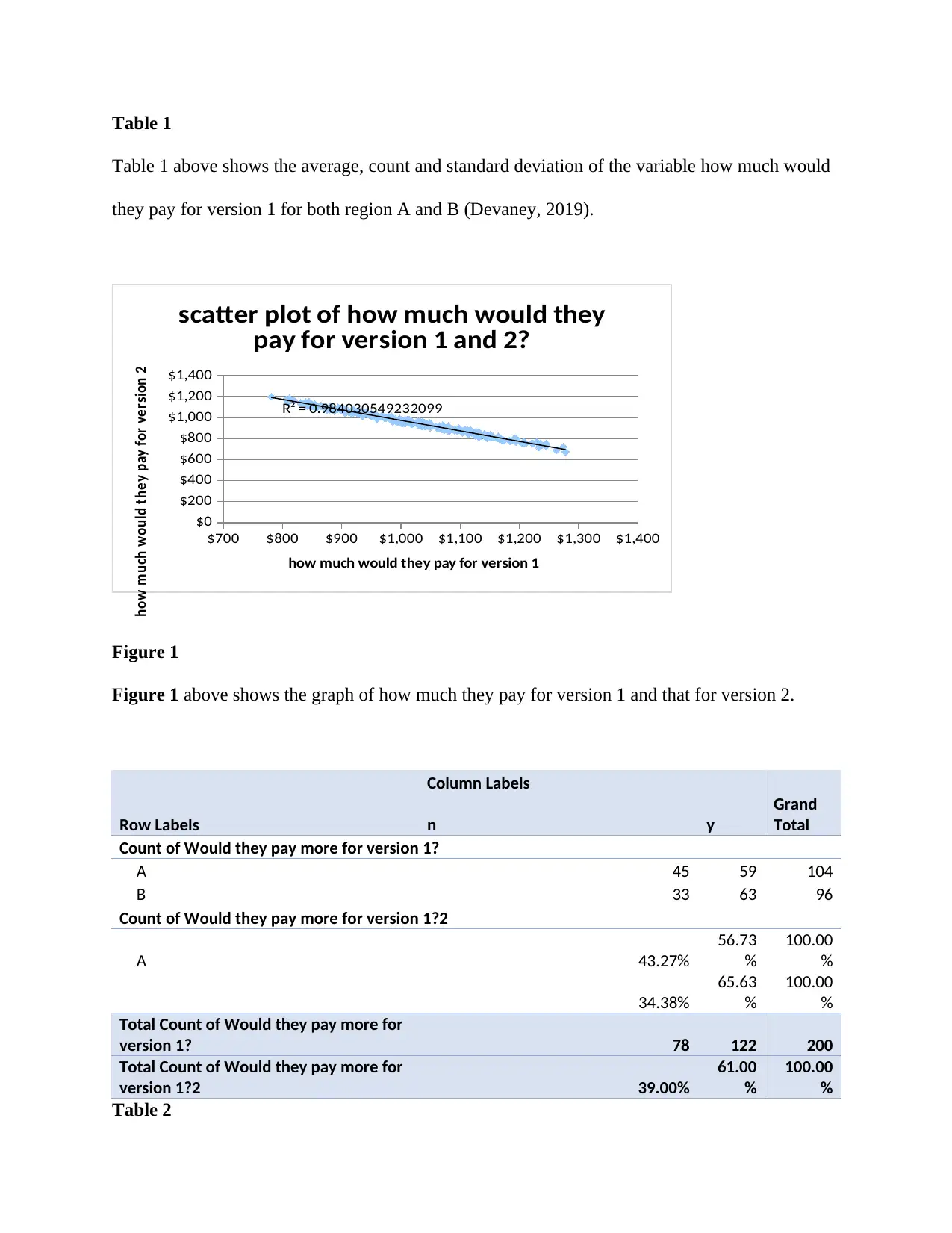
Table 1
Table 1 above shows the average, count and standard deviation of the variable how much would
they pay for version 1 for both region A and B (Devaney, 2019).
$700 $800 $900 $1,000 $1,100 $1,200 $1,300 $1,400
$0
$200
$400
$600
$800
$1,000
$1,200
$1,400
R² = 0.984030549232099
scatter plot of how much would they
pay for version 1 and 2?
how much would they pay for version 1
how much would they pay for version 2
Figure 1
Figure 1 above shows the graph of how much they pay for version 1 and that for version 2.
Column Labels
Row Labels n y
Grand
Total
Count of Would they pay more for version 1?
A 45 59 104
B 33 63 96
Count of Would they pay more for version 1?2
A 43.27%
56.73
%
100.00
%
34.38%
65.63
%
100.00
%
Total Count of Would they pay more for
version 1? 78 122 200
Total Count of Would they pay more for
version 1?2 39.00%
61.00
%
100.00
%
Table 2

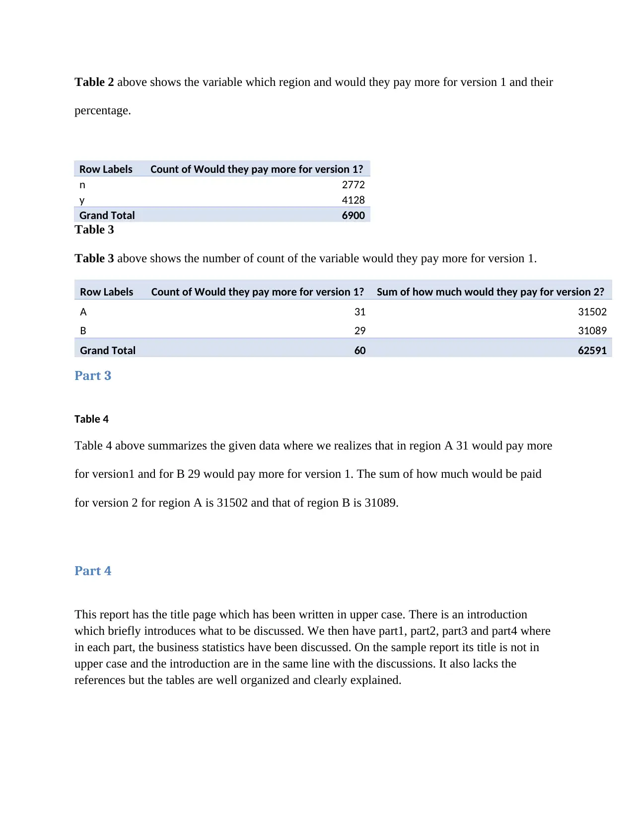
Table 2 above shows the variable which region and would they pay more for version 1 and their
percentage.
Row Labels Count of Would they pay more for version 1?
n 2772
y 4128
Grand Total 6900
Table 3
Table 3 above shows the number of count of the variable would they pay more for version 1.
Row Labels Count of Would they pay more for version 1? Sum of how much would they pay for version 2?
A 31 31502
B 29 31089
Grand Total 60 62591
Part 3
Table 4
Table 4 above summarizes the given data where we realizes that in region A 31 would pay more
for version1 and for B 29 would pay more for version 1. The sum of how much would be paid
for version 2 for region A is 31502 and that of region B is 31089.
Part 4
This report has the title page which has been written in upper case. There is an introduction
which briefly introduces what to be discussed. We then have part1, part2, part3 and part4 where
in each part, the business statistics have been discussed. On the sample report its title is not in
upper case and the introduction are in the same line with the discussions. It also lacks the
references but the tables are well organized and clearly explained.

References
Cameron, C. (2009). EXCEL Multiple Regressions. [online] Cameron.econ.ucdavis.edu.
Available at: http://cameron.econ.ucdavis.edu/excel/ex61multipleregression.html [Accessed 27
May 2019].
Devaney, E. (2019). HubSpot Blogs | Marketing | Erik Devaney. [online] Blog.hubspot.com.
Available at: https://blog.hubspot.com/marketing/author/erik-devaney [Accessed 27 May 2019].