Control Design for F-18 Longitudinal Dynamics

This document discusses the control design for F-18 Longitudinal Dynamics. It covers topics such as open loop system modes, transfer function, equivalent compensator, root locus and system controllability. The document also provides MATLAB code for computations. The subject is Control Design and the course code is F-18 Longitudinal Dynamics. The document is relevant for students studying this course at any college or university.

Student Name
Student ID Number
CONTROL DESIGN
Institutional Affiliation
F-18 Longitudinal Dynamics
Assignment
Date of submission
Question 1
2018

Open loop system modes
A system can be represented using the continuous time domain function or using
the state space. The state space uses matrix notation to represent a system of
signals. The standard state space representation is,
˙x= Ax+ Bu
y=Cx + Du
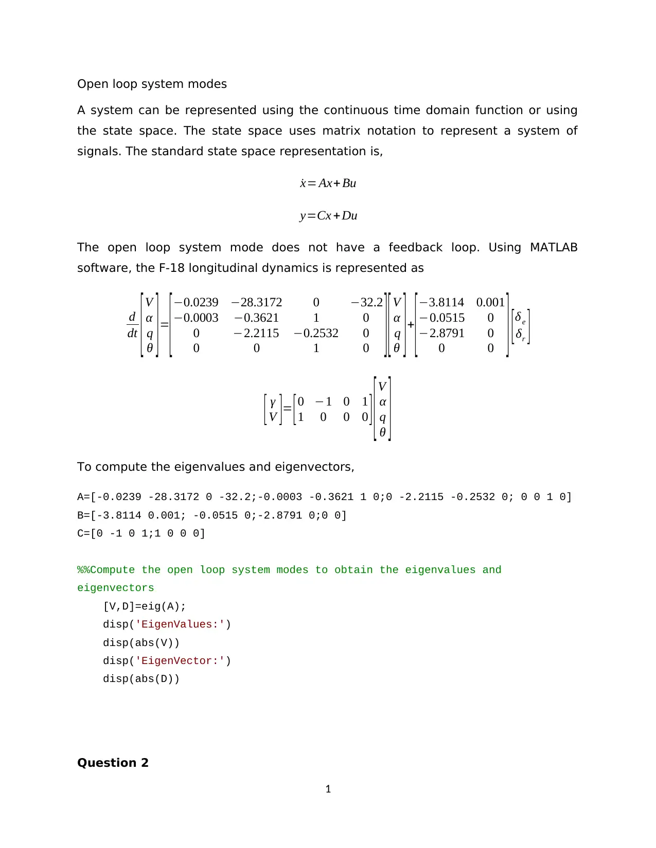
The open loop system mode does not have a feedback loop. Using MATLAB
software, the F-18 longitudinal dynamics is represented as
d
dt [ V
α
q
θ ] =
[ −0.0239 −28.3172 0 −32.2
−0.0003 −0.3621 1 0
0 −2.2115 −0.2532 0
0 0 1 0 ][ V
α
q
θ ] +
[ −3.8114 0.001
−0.0515 0
−2.8791 0
0 0 ] [ δe
δr ]
[ γ
V ]= [ 0 −1 0 1
1 0 0 0 ] [ V
α
q
θ ]
To compute the eigenvalues and eigenvectors,
A=[-0.0239 -28.3172 0 -32.2;-0.0003 -0.3621 1 0;0 -2.2115 -0.2532 0; 0 0 1 0]
B=[-3.8114 0.001; -0.0515 0;-2.8791 0;0 0]
C=[0 -1 0 1;1 0 0 0]
%%Compute the open loop system modes to obtain the eigenvalues and
eigenvectors
[V,D]=eig(A);
disp('EigenValues:')
disp(abs(V))
disp('EigenVector:')
disp(abs(D))
Question 2
1

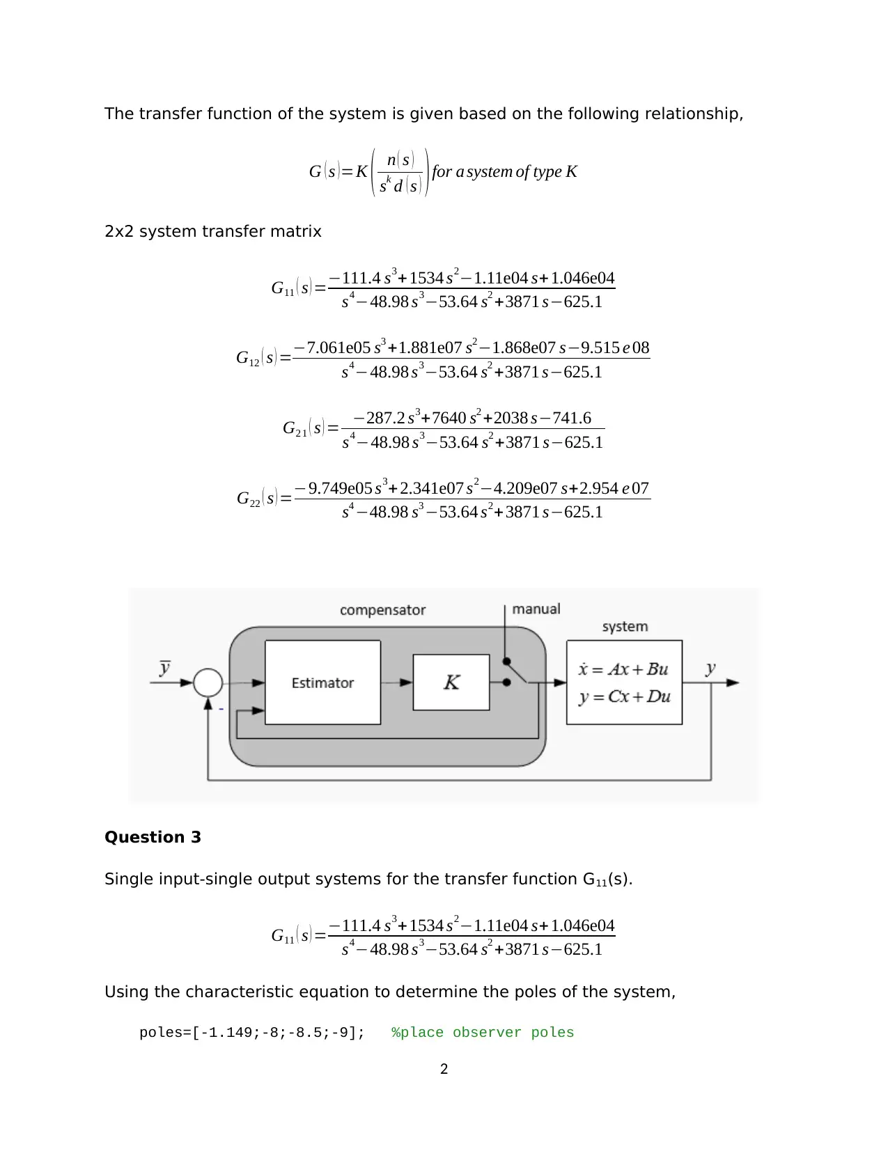
The transfer function of the system is given based on the following relationship,
G ( s )=K ( n ( s )
sk d ( s ) )for a system of type K
2x2 system transfer matrix
G11 ( s ) =−111.4 s3+1534 s2−1.11e04 s+1.046e04
s4−48.98 s3−53.64 s2 +3871 s−625.1
G12 ( s ) =−7.061e05 s3 +1.881e07 s2−1.868e07 s−9.515 e 08
s4−48.98 s3−53.64 s2 +3871 s−625.1
G2 1 ( s ) = −287.2 s3+7640 s2 +2038 s−741.6
s4−48.98 s3−53.64 s2 +3871 s−625.1
G22 ( s ) =−9.749e05 s3+ 2.341e07 s2−4.209e07 s+2.954 e 07
s4 −48.98 s3 −53.64 s2+3871 s−625.1
Question 3
Single input-single output systems for the transfer function G11(s).
G11 ( s ) =−111.4 s3+1534 s2−1.11e04 s+1.046e04
s4−48.98 s3−53.64 s2 +3871 s−625.1
Using the characteristic equation to determine the poles of the system,
poles=[-1.149;-8;-8.5;-9]; %place observer poles
2

% To determine the equivalent compensator for the Open Loop system
...transfer function.
Gcss=ss(Ac,Bc,Cc,0);
Gc=tf(Gcss);
zpk(Gc)
Question 4
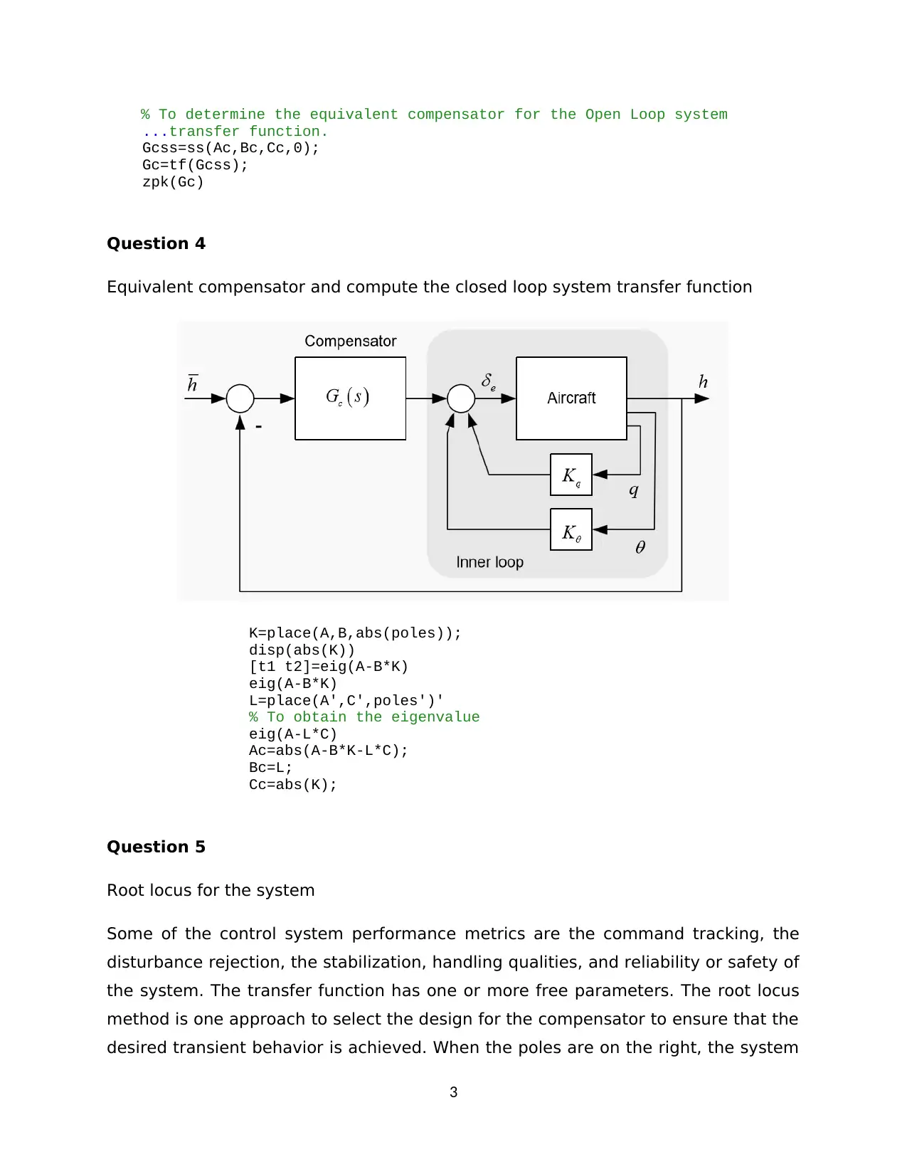
Equivalent compensator and compute the closed loop system transfer function
K=place(A,B,abs(poles));
disp(abs(K))
[t1 t2]=eig(A-B*K)
eig(A-B*K)
L=place(A',C',poles')'
% To obtain the eigenvalue
eig(A-L*C)
Ac=abs(A-B*K-L*C);
Bc=L;
Cc=abs(K);
Question 5
Root locus for the system
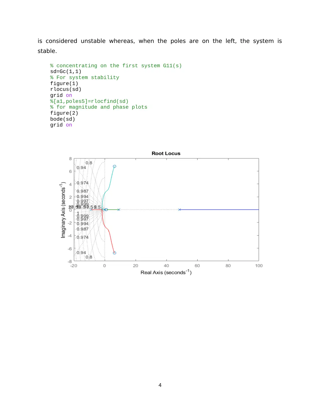
Some of the control system performance metrics are the command tracking, the
disturbance rejection, the stabilization, handling qualities, and reliability or safety of
the system. The transfer function has one or more free parameters. The root locus
method is one approach to select the design for the compensator to ensure that the
desired transient behavior is achieved. When the poles are on the right, the system
3

is considered unstable whereas, when the poles are on the left, the system is
stable.
% concentrating on the first system G11(s)
sd=Gc(1,1)
% For system stability
figure(1)
rlocus(sd)
grid on
%[a1,poles5]=rlocfind(sd)
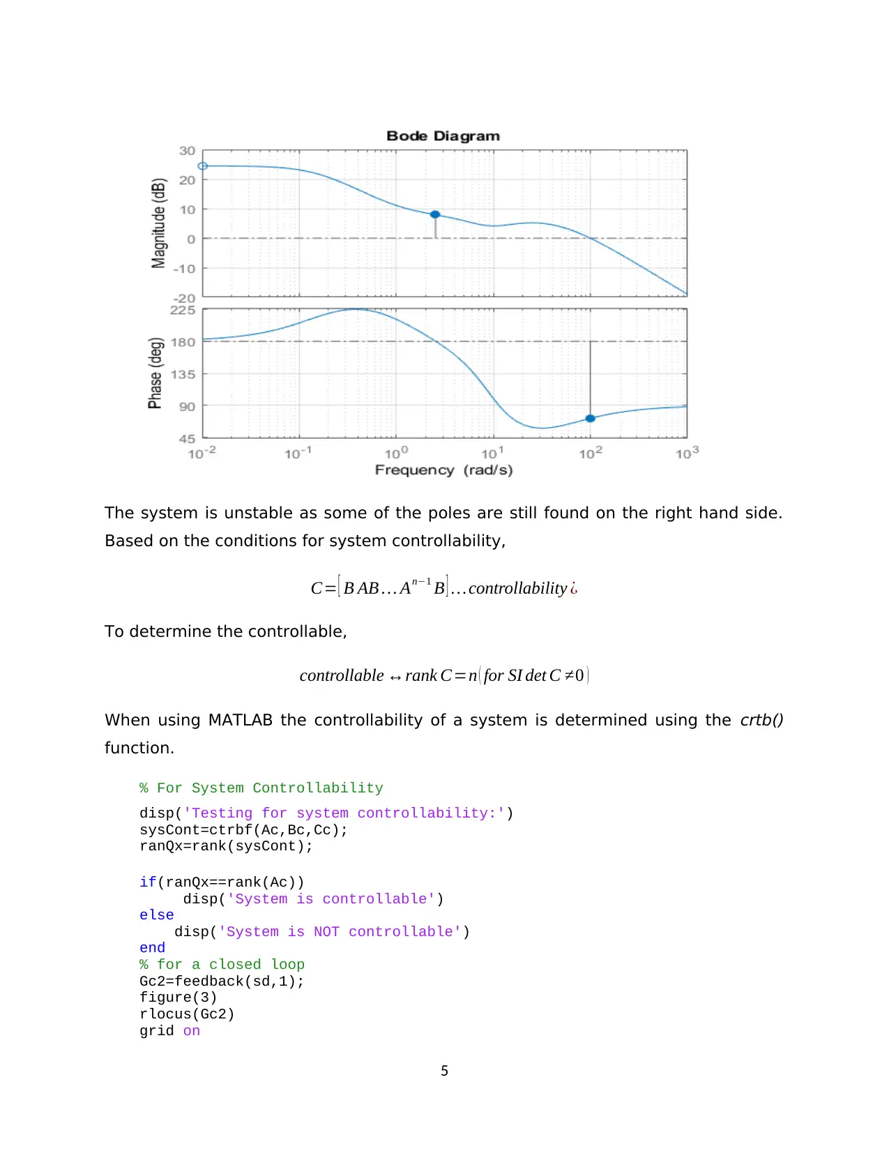
% for magnitude and phase plots
figure(2)
bode(sd)
grid on
4

The system is unstable as some of the poles are still found on the right hand side.
Based on the conditions for system controllability,
C= [ B AB … An−1 B ] … controllability ¿
To determine the controllable,
controllable ↔rank C=n ( for SI det C ≠0 )
When using MATLAB the controllability of a system is determined using the crtb()
function.
% For System Controllability
disp('Testing for system controllability:')
sysCont=ctrbf(Ac,Bc,Cc);
ranQx=rank(sysCont);
if(ranQx==rank(Ac))
disp('System is controllable')
else
disp('System is NOT controllable')
end
% for a closed loop
Gc2=feedback(sd,1);
figure(3)
rlocus(Gc2)
grid on
5