Control Systems: Feedback Analysis and Design - Assignment

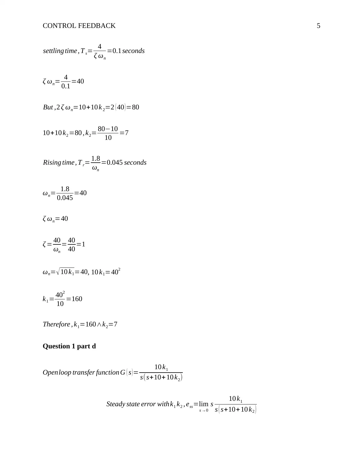
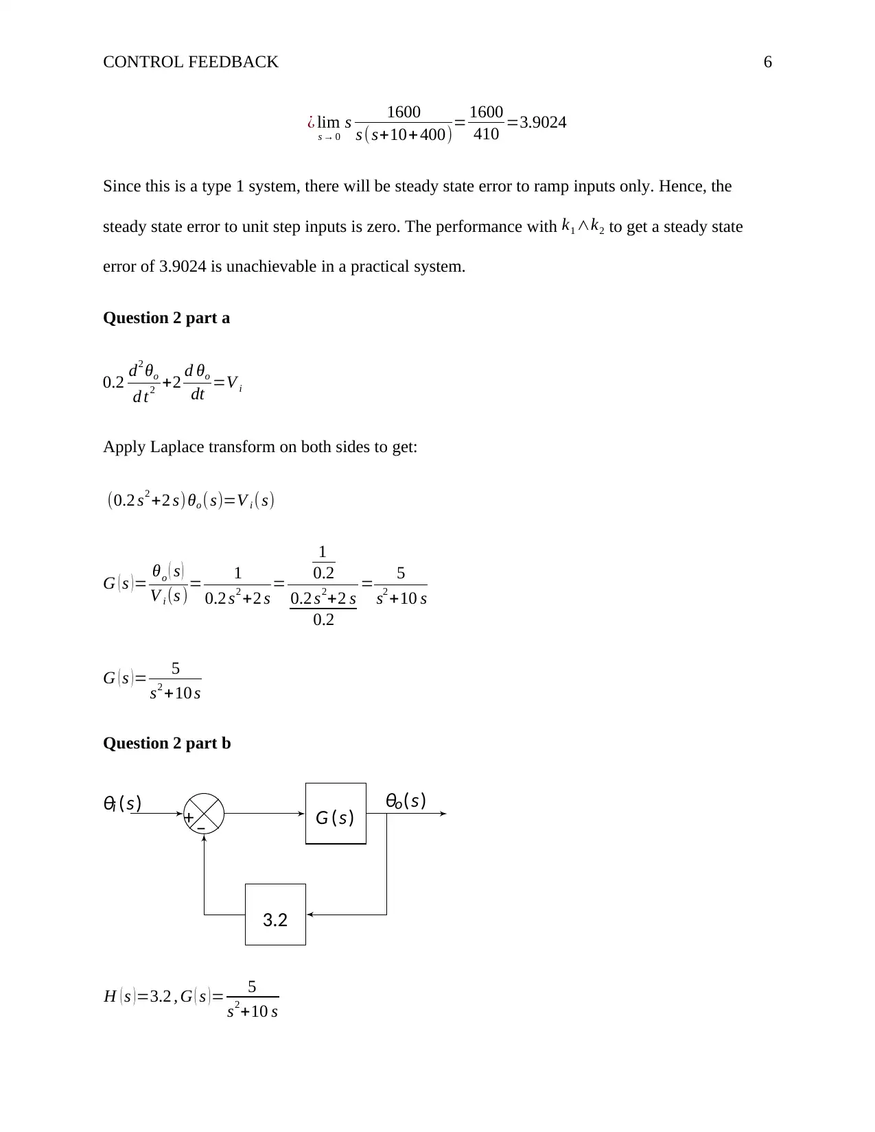
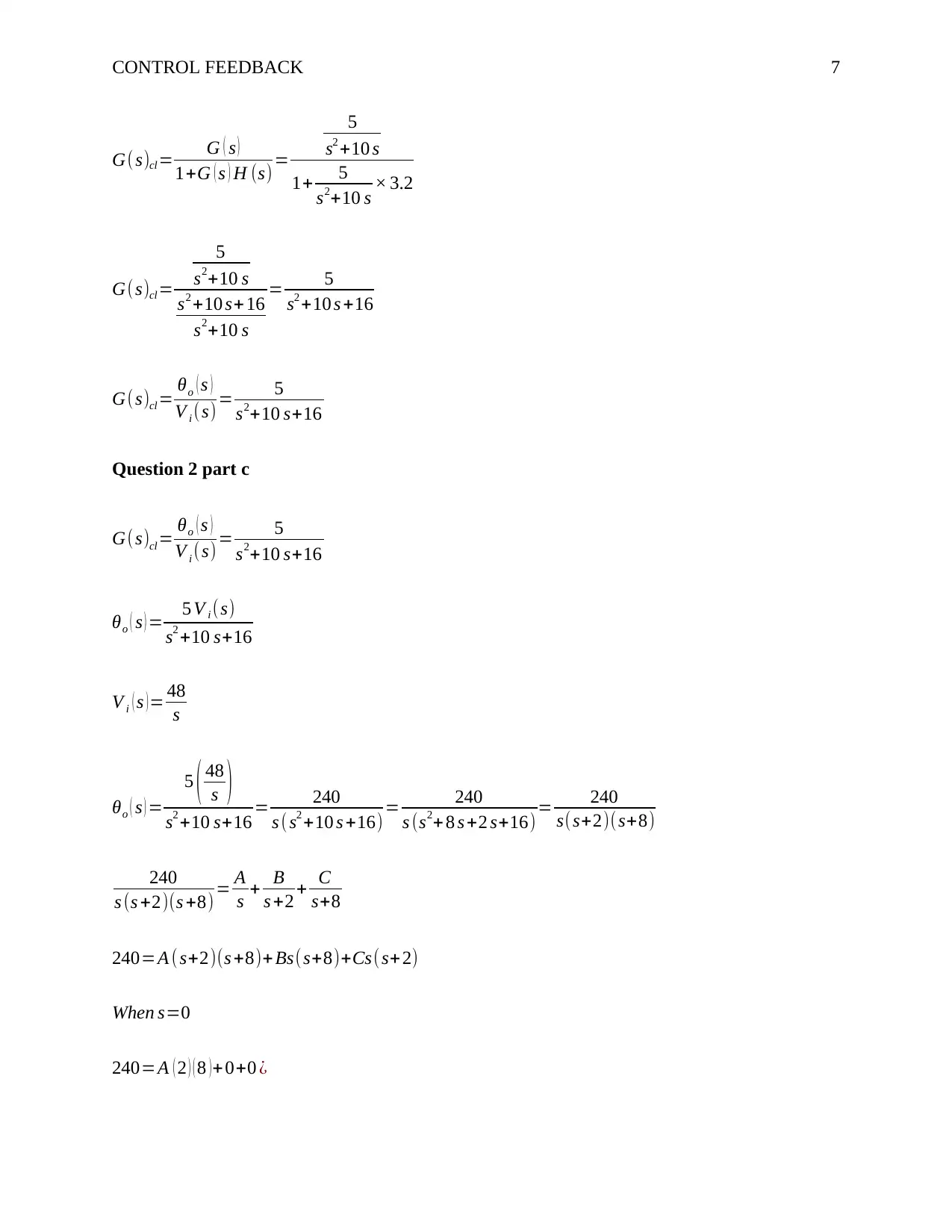
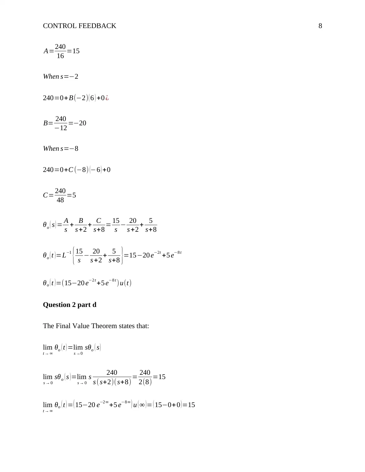
This document provides a comprehensive solution to a control feedback analysis assignment. The solution covers various aspects of control systems, including the analysis and design of feedback loops. It begins with determining system parameters (k and p) based on step response characterist...Read More

Running head: CONTROL FEEDBACK 1
Control Feedback
Name
Institution

CONTROL FEEDBACK 2
Control Feedback
Question 1 part a
Openloop transfer function ,G ( s )=10 × 1
s × k
(s + p) = 10 k
s( s+ p)
Closed looptransfer function ,= G ( s )
1+G ( s ) H (s)=
10 k
s ( s+ p)
1+ 10 k
s(s + p)
Closed looptransfer function=
10 k
s (s + p)
s (s+ p)+10 k
s (s + p)
= 10 k
s2 +sp+10 k
The transfer function is in the form:
ωn
2
s2+ 2ζ ωn s+ωn
2
ωn= √ 10 k , 2ζ ωn= p
Maximum % peak overshoop , M p=e
−π ζ
√1−ζ 2
× 100 %=16.3 %
e
−π ζ
√ 1−ζ 2
=0.163
ln e
−π ζ
√ 1−ζ 2
=ln 0.163
π ζ
√ 1−ζ2 =ln 0.163
π2 ζ2
1−ζ2 = ( ln0.163 )2

CONTROL FEEDBACK 3
π2 ζ2= ( ln0.163 )2 − ( ln 0.1632 ) 2 ζ 2
π2 ζ2+ ( ln 0.163 ) 2 ζ 2= ( ln 0.163 )2
ζ 2 ( π2 + ( ln 0.163 )2 )= ( ln 0.163 )2
ζ = √ ( ln 0.163 )2
π2 + ( ln 0.163 )2 =0.5
settling time, T s= 4
ζ ωn
=0.8 seconds
4
0.5 ωn
=0.8
ωn= 4
0.5 ×0.8 =10
ωn= √ 10 k
p=2ζ ωn=2 ×0.5 ×10=10
ωn= √ 10 k=10
10 k =102=100
k =100
10 =10
Therefore , k= p=10
Question 1 part b

CONTROL FEEDBACK 4
G ( s )
1+ G ( s ) H (s) =
k
s+ p
1+ k k2
s + p
=
k
s+ p
s + p+k k2
s+ p
= k
s+ p+k k2
Openloop transfer function , θo (s)
θi ( s) = k
s +p +k k2
( k1 ) ( 1
s )= k k 1
s ( s + p+k k2 )
Plugging k= p=10 yields:
Openloop transfer function , θo (s)
θi ( s) = 10 k1
s2+ 10 s+10 k2 s
Closed looptransfer function , θo (s )
θi (s) =
10 k1
s2 +10 s +10 k2 s
1+ 10 k1
s2+ 10 s+10 k2 s
= 10 k1
s2+10 s+10 k2 s +10 k1
Closed looptransfer function , θo (s )
θi (s) = 10 k1
s2 +(10+10 k2) s+10 k1
Question 1 part c
The transfer function , 10 k1
s2 +(10+10 k2 )s+10 k1
is∈the form ωn
2
s2+ 2ζ ωn s+ ωn
2
ωn= √10 k1 ,2 ζ ωn=10+10 k2
−
+
θi (s) k1 −
+ k
(s + p)
k2
1
s
θo(s)

CONTROL FEEDBACK 5
settling time, T s= 4
ζ ωn
=0.1 seconds
ζ ωn= 4
0.1 =40
But ,2 ζ ωn=10+10 k 2=2 ( 40 )=80
10+10 k2 =80 , k2= 80−10
10 =7
Rising time, T r= 1.8
ωn
=0.045 seconds
ωn= 1.8
0.045 =40
ζ ωn=40
ζ = 40
ωn
= 40
40 =1
ωn= √10 k1=40, 10 k1=402
k1 = 402
10 =160
Therefore , k1=160∧k2=7
Question 1 part d
Openloop transfer function G ( s ) = 10 k1
s(s+10+ 10 k2)
Steady state error withk1 k2 , ess=lim
s →0
s 10 k1
s ( s+10+10 k2 )

CONTROL FEEDBACK 6
¿ lim
s → 0
s 1600
s ( s+10+ 400)= 1600
410 =3.9024
Since this is a type 1 system, there will be steady state error to ramp inputs only. Hence, the
steady state error to unit step inputs is zero. The performance with k1 ∧k2 to get a steady state
error of 3.9024 is unachievable in a practical system.
Question 2 part a
0.2 d2 θo
d t2 +2 d θo
dt =V i
Apply Laplace transform on both sides to get:
(0.2 s2 +2 s)θo (s)=V i (s)
G ( s ) = θo ( s )
V i (s )= 1
0.2 s2 +2 s =
1
0.2
0.2 s2+2 s
0.2
= 5
s2 +10 s
G ( s )= 5
s2 +10 s
Question 2 part b
H ( s )=3.2 , G ( s )= 5
s2+10 s
−
+ G (s)
3.2
θi (s) θo(s)

CONTROL FEEDBACK 7
G(s)cl = G ( s )
1+G ( s ) H (s)=
5
s2 +10 s
1+ 5
s2+10 s × 3.2
G(s)cl =
5
s2+10 s
s2 +10 s+ 16
s2+10 s
= 5
s2 +10 s +16
G(s)cl = θo ( s )
V i (s)= 5
s2+10 s+16
Question 2 part c
G(s)cl = θo ( s )
V i (s)= 5
s2+10 s+16
θo ( s ) = 5 V i (s)
s2 +10 s+16
V i ( s )= 48
s
θo ( s ) =
5 ( 48
s )
s2 +10 s+16 = 240
s ( s2 +10 s +16) = 240
s (s2+ 8 s +2 s+16)= 240
s(s+2)(s+8)
240
s (s +2)(s +8) = A
s + B
s +2 + C
s+8
240=A ( s+2)(s +8)+ Bs(s+8)+Cs( s+2)
When s=0
240=A ( 2 ) ( 8 )+ 0+0 ¿

CONTROL FEEDBACK 8
A=240
16 =15
When s=−2
240=0+ B(−2) ( 6 ) +0 ¿
B= 240
−12 =−20
When s=−8
240=0+C (−8) (−6 ) +0
C= 240
48 =5
θo ( s ) = A
s + B
s +2 + C
s+8 = 15
s − 20
s +2 + 5
s+8
θo ( t )=L−1
{15
s − 20
s +2 + 5
s+8 }=15−20 e−2t +5 e−8 t
θo ( t ) =(15−20 e−2 t +5 e−8 t )u(t)
Question 2 part d
The Final Value Theorem states that:
lim
t → ∞
θo ( t ) =lim
s →0
sθo ( s )
lim
s → 0
sθo ( s ) =lim
s → 0
s 240
s (s+2)( s+8)= 240
2(8)=15
lim
t → ∞
θo ( t ) = ( 15−20 e−2 ∞ +5 e−8 ∞ ) u ( ∞ )= ( 15−0+0 )=15

CONTROL FEEDBACK 9
Therefore , lim
t → ∞
θo ( t )=lim
s → 0
sθo ( s )
The steady output does not match the input in part (c) because the servomechanism does not
have a unity feedback.
Question 2 part e
Increasing the gain parameters from 3.2 increases the response of the system. However,
increasing the value beyond a particular safety zone could make the system unstable. Introducing
an integral and differential control into the system could increase the steady-state output for the
same magnitude input step without affecting response speed.
Question 3 part a
The Nyquist plot using the given data points is shown below.

CONTROL FEEDBACK 10
The suitabletransfer function is 100
9 s2 +7 s+10
The MATLAB code for drawing the Nyquist diagram based on the transfer function is:
%MATLAB code for drawing Nyquist from the transfer function
num=[100];
den=[9 7 10];
G=tf(num,den);%transfer function
nyquist(G)

CONTROL FEEDBACK 11
Question 3 part b
Transfer function= 100
−9 ω2 + j 7 ω +10 = 100
( 10−9 ω2 ) + j 7 ω
The magnitude=20 log 100
√ ( 10−9 ω2 )2
+49 ω2
dB
The phase of the system=−tan−1
( 7 ω
10−9 ω2 )
%MATLAB code for calculating magnitude and phase
omega=1.2
mag=20*log10(100/(sqrt((10-9*omega^2)^2+49*omega^2)))
Phase_a=-atan(7*omega/(10-9*omega^2));
Phase=Phase_a*180/pi

CONTROL FEEDBACK 12
Running the MATLAB code gives the results below :
Question 3 part c
The closed loop system will have a pole on the negative half s-plane making it instable.
k = 5 would give a phase margin of 30◦.

CONTROL FEEDBACK 13
The phase margin is 15 degrees while the gain margin is:
GM =1
2 =0.5
The steady state error will be zero.
Question 4 part a
The open loop transfer function becomes:
θo ( s )
θi ( s ) = 4 K
( s+1 ) ( s+5 ) = 4 k
s2 +6 s +5
−
+
θi (s) K (s) G (s)= 4
s(s +1) ( s +5)
θo(s)

CONTROL FEEDBACK 14
The function is∈the form ωn
2
s2 +2 ζ ωn s +ωn
2
ωn= √4 k ,2 ζ ωn=6 , ζ ωn= 6
2 =3
settling time, T s ≤ 4
ζ ωn
=1.7 seconds
ζ ωn ≥ 4
1.7 ≥ 2.3529
θo ( jω )
θi ( jω ) = 4 k
( jω+1 ) ( jω+5 ) = 4 k
−ω2 + j6 ω +5 = 4 k
( 5−ω2 ) + j 6 ω
The magnitude ,
|θo ( jω )
θi ( jω ) |= 4
√ ( 5−ω2 ) 2
+ 36 ω2
The phase of the system=−tan−1
( 6 ω
5−ω2 )
The resonant peak , M r = 1
2 ζ √1−ζ2 =31 dB(¿ the Bode plot)
Question 4 part b
The transfer function of uncompensated system is:
θo ( s )
θi ( s ) = 4 K
( s+1 ) ( s+5 ) = 4
s2 +6 s +5
Gain crossover frequency is the frequency at which the magnitude plot crosses the 0dB line.

CONTROL FEEDBACK 15
Gain cross−¿ frequency =0.7 rad s−1
The compensator transfer function is ,C ( s )= 1+ a Ts
1+ Ts
Phase margin of uncompensated system ¿−135° +180 °=45 °
Gain margin of uncompensated system ¿ 18 dB
Phase margin of compensated system ¿−13 0° +180 °=50 °
Gain margin of compensated system ¿ 1 6 dB
ϕm =50−45=5 °
sin ϕm =sin 5=0.08716= a−1
a+1
0.08716 a+0.08716=a−1

CONTROL FEEDBACK 16
a=1.191
ωm=−10 loga=−10 log 1.191=−0.759
Compensator pole , p=ωm √a=−0.759 √ 1.191=−0.828
Compensator zero , z=− p
a = 0.828
1.191 =0.695
Compensator transfer function= s−0.695
s +0.828
¿
1
−0.695 (1−0.695 s)
1
0.828 (1+ 828 s)
=−1.191 1−0.695 s
1+ 0.828 s
Compensator transfer function=−1.191 1−0.695 s
1+0.828 s
Question 4 part c
The MATLAB code is shown below:
%MATLAB code showing the gain and phase margin of compensated system
num=[4]
den=[1 6 5]
G=tf(num,den);%transfer function uncompensated system
numc=-1.191*[-0.695 1];
denc=[0.828 1];
Gc=tf(numc,denc);%transfer function compensated system
L=series(G,Gc);
bode(L)
grid
[Gm,Pm,wpm,wgm]=margin(L);
GmdB=20*log10(Gm);
[Gm,Pm,wpm,wgm]
The resulting output is:

CONTROL FEEDBACK 17
%MATLAB code for the closed loop transfer function
num=[4]
den=[1 6 5]
G=tf(num,den);%transfer function uncompensated system
numc=1.191*[-0.695 1];
denc=[0.828 1];
Gc=tf(numc,denc);

CONTROL FEEDBACK 18
L=series(G,Gc);%transfer function compensated system
H=feedback(L,1);%closed loop transfer function
step(H)
The resulting output is:
Question 4 part d
If the settling time is halved whilst maintaining the same damping ratio, the design will not work.
settling time, T s ≤ 4
ζ ωn
= 1.7
2 =0.85 seconds
The design is not possible since halving the settling time affects the damping ratio. The
compensator could be modified to enable a successful design by changing the damping ratio to
the appropriate limits.

CONTROL FEEDBACK 19
Question 4 part e
steady state error=lim
s → 0
sG ( s ) =lim
s →0
¿ 4
s2+ 6 s+ 5 × s−0.695
s+0.828 = 4
5 × −0.695
0.828 =−0.6715
To reduce this steady-state error, a PID controller could be the best choice as it will cater for
both the frequency response and the steady state error.