Ask a question from expert
Control & Instrumentation PDF
25 Pages2647 Words97 Views
Added on 2021-11-03
Control & Instrumentation PDF
Added on 2021-11-03
BookmarkShareRelated Documents
Control & InstrumentationLab Assignment
Student Name
Student ID Number
Instructor (professor)
Institutional affiliation
Location(state, country)
Date of submission
Student Name
Student ID Number
Instructor (professor)
Institutional affiliation
Location(state, country)
Date of submission

TABLE OF CONTENTS
INTRODUCTION...........................................................................................................................1
AIMS OF THE EXPERIMENT......................................................................................................3
ROTARY INVERTED PENDULUM SYSTEM MODEL.............................................................3
ROTARY INVERTED PENDULUM SIMULINK MODEL.........................................................7
CONTROLLER DESIGN...............................................................................................................8
DISCUSSION..................................................................................................................................8
CONCLUSION & FUTURE WORKS...........................................................................................8
REFERENCES................................................................................................................................9
LIST OF FIGURES
Figure 1 ROTPEN rotary inverted pendulum on LABVIEW [source: Quanser].........................................3
Figure 2 Free body diagram of the rotary inverted pendulum......................................................................4
Figure 3ROTPEN Matlab Simulink Model-Overview................................................................................9
Figure 4 Step response ROTPEN Matlab Simulink Model Output............................................................12
Figure 5 Bode Diagram to show magnitude and phase of ROTPEN Pendulum........................................13
Figure 6 Open loop system Simulation Model Block................................................................................14
Figure 7 Root Locus for Transfer Function 1............................................................................................15
Figure 8 Root Locus for transfer function 2...............................................................................................16
Figure 9 Pole location for a closed loop system........................................................................................18
Figure 10 State feedback controller for a closed loop ROTPEN pendulum...............................................18
Figure 11 The ROTPEN controller for the Pendulum link........................................................................19
Figure 12 System Simulation Balance Control Response for the closed loop............................................20
Figure 13 Results form Simulation of the ROTPEN model.......................................................................21
Figure 14 ROTPEN Model........................................................................................................................22
Figure 15 State Feedback controller segment............................................................................................22
1 | Page
INTRODUCTION
The rotary inverted pendulum is a nonlinear system whose initial state is unstable hence
the need for control. There are different methods implemented in the control of the rotary
inverted pendulum. In the analysis, the velocity of the pendulum center of mass, is considered for
a system displaced in the angle, a, and in the x-direction [1]-[5]. The system has a motor that
moves the cart along a straight track with the pendulum attached to the cart using a pin joint. The
axis of rotation of the pendulum link is considered to be horizontal and it is perpendicular to the
cart’s direction of motion. The input of the system is the force that is applied to the cart through
the motor. The horizontal link is coupled such that it links directly or by connecting to a gearing
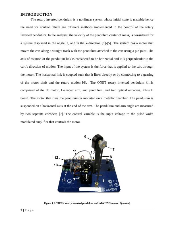
of the motor shaft and the rotary motion [6]. The QNET rotary inverted pendulum kit is
comprised of the dc motor, L-shaped arm, and pendulum, and two optical encoders, Elvis II
board. The motor that runs the pendulum is mounted on a metallic chamber. The pendulum is
suspended on a horizontal axis at the end of the arm. The pendulum and arm angle are measured
by two separate encoders [7]. The control variable is the input voltage to the pulse width
modulated amplifier that controls the motor.
Figure 1 ROTPEN rotary inverted pendulum on LABVIEW [source: Quanser]
2 | Page
The rotary inverted pendulum is a nonlinear system whose initial state is unstable hence
the need for control. There are different methods implemented in the control of the rotary
inverted pendulum. In the analysis, the velocity of the pendulum center of mass, is considered for
a system displaced in the angle, a, and in the x-direction [1]-[5]. The system has a motor that
moves the cart along a straight track with the pendulum attached to the cart using a pin joint. The
axis of rotation of the pendulum link is considered to be horizontal and it is perpendicular to the
cart’s direction of motion. The input of the system is the force that is applied to the cart through
the motor. The horizontal link is coupled such that it links directly or by connecting to a gearing
of the motor shaft and the rotary motion [6]. The QNET rotary inverted pendulum kit is
comprised of the dc motor, L-shaped arm, and pendulum, and two optical encoders, Elvis II
board. The motor that runs the pendulum is mounted on a metallic chamber. The pendulum is
suspended on a horizontal axis at the end of the arm. The pendulum and arm angle are measured
by two separate encoders [7]. The control variable is the input voltage to the pulse width
modulated amplifier that controls the motor.
Figure 1 ROTPEN rotary inverted pendulum on LABVIEW [source: Quanser]
2 | Page
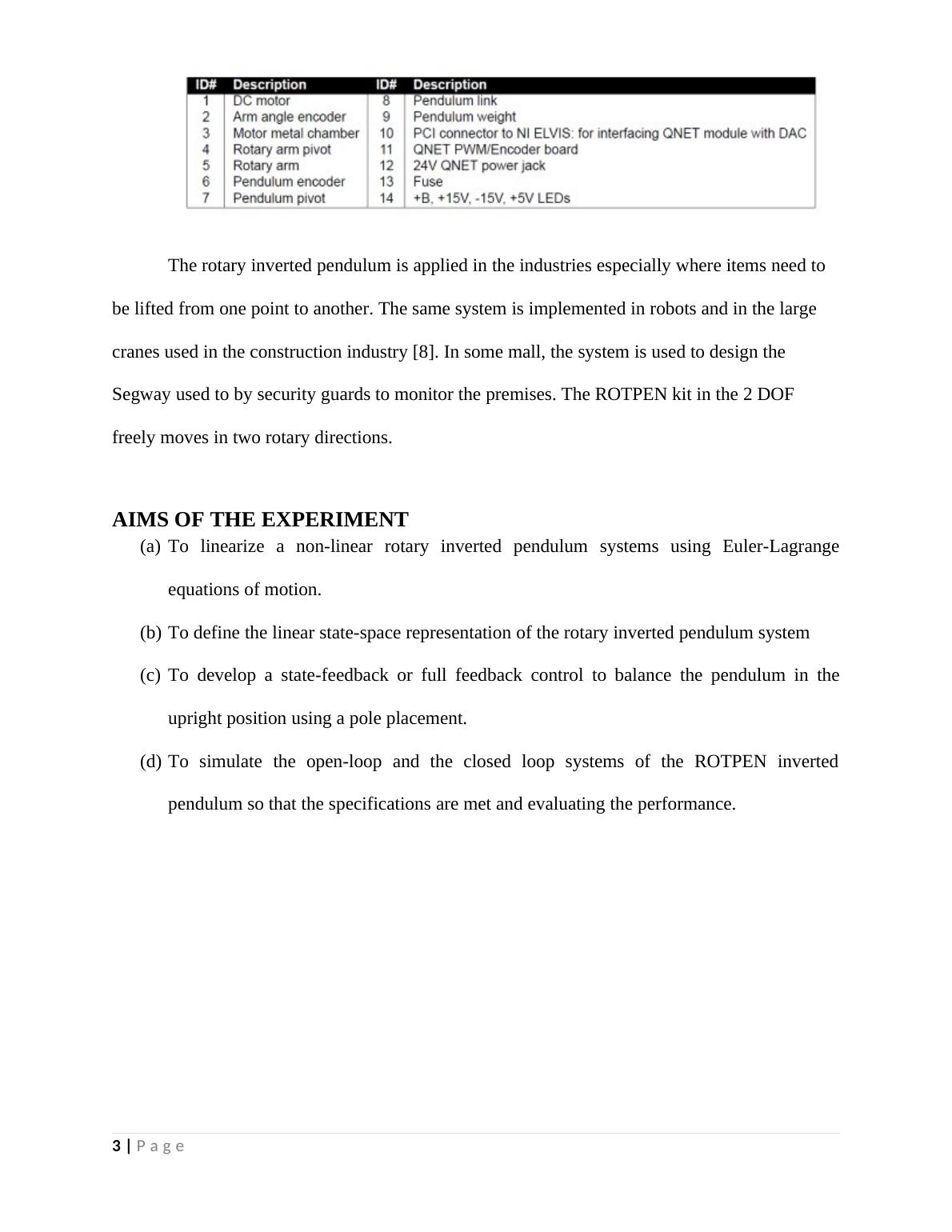
The rotary inverted pendulum is applied in the industries especially where items need to
be lifted from one point to another. The same system is implemented in robots and in the large
cranes used in the construction industry [8]. In some mall, the system is used to design the
Segway used to by security guards to monitor the premises. The ROTPEN kit in the 2 DOF
freely moves in two rotary directions.
AIMS OF THE EXPERIMENT
(a) To linearize a non-linear rotary inverted pendulum systems using Euler-Lagrange
equations of motion.
(b) To define the linear state-space representation of the rotary inverted pendulum system
(c) To develop a state-feedback or full feedback control to balance the pendulum in the
upright position using a pole placement.
(d) To simulate the open-loop and the closed loop systems of the ROTPEN inverted
pendulum so that the specifications are met and evaluating the performance.
3 | Page
ROTARY INVERTED PENDULUM SYSTEM MODEL
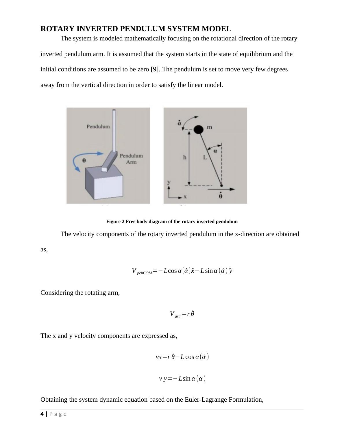
The system is modeled mathematically focusing on the rotational direction of the rotary
inverted pendulum arm. It is assumed that the system starts in the state of equilibrium and the
initial conditions are assumed to be zero [9]. The pendulum is set to move very few degrees
away from the vertical direction in order to satisfy the linear model.
Figure 2 Free body diagram of the rotary inverted pendulum
The velocity components of the rotary inverted pendulum in the x-direction are obtained
as,
V penCOM=−Lcosα ( ̇α )^x−Lsinα ( ̇α)^y
Considering the rotating arm,
Varm=r ̇θ
The x and y velocity components are expressed as,
vx=r ̇θ−Lcosα( ̇α )
v y=−Lsinα ( ̇α )
Obtaining the system dynamic equation based on the Euler-Lagrange Formulation,
4 | Page
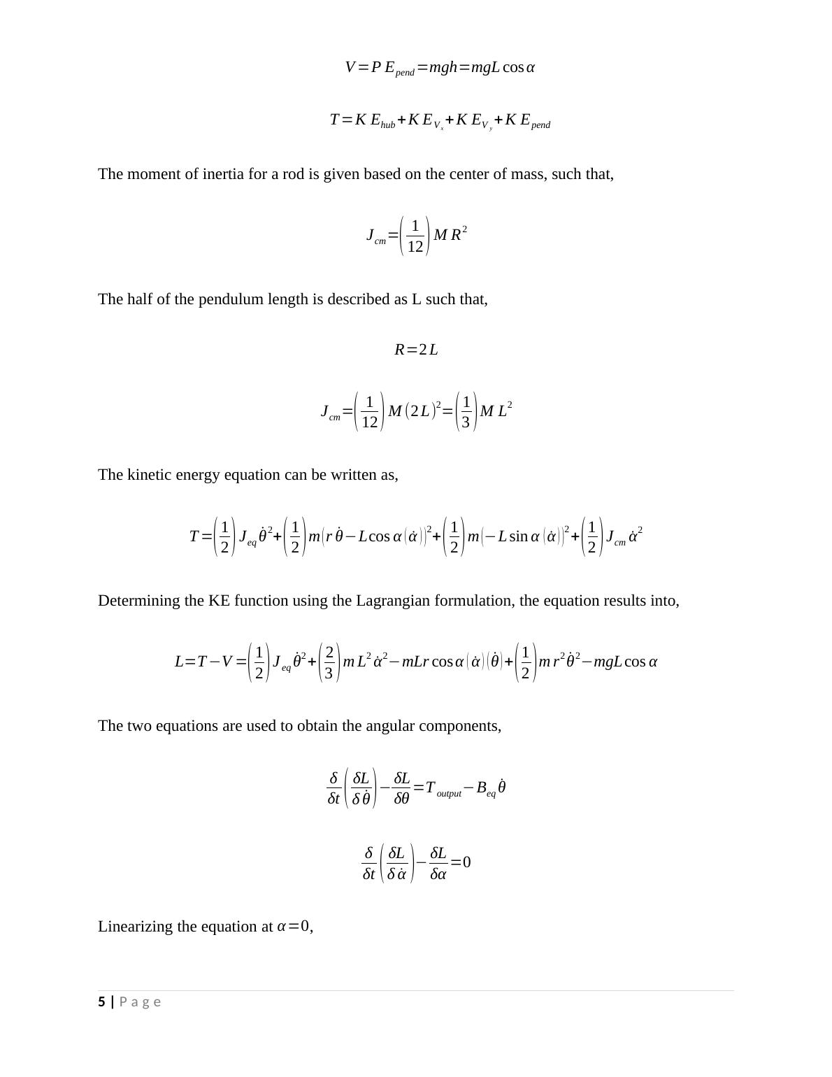
V=P Epend=mgh=mgL cosα
T=K Ehub +K EVx
+K EV y
+K Epend
The moment of inertia for a rod is given based on the center of mass, such that,
Jcm=(1
12)M R2
The half of the pendulum length is described as L such that,
R=2L
Jcm=(1
12)M (2L)2=(1
3)M L2
The kinetic energy equation can be written as,
T=(1
2)Jeq ̇θ2+(1
2)m(r ̇θ−Lcosα ( ̇α ))2+(1
2)m(−Lsinα ( ̇α))2+(1
2)Jcm ̇α2
Determining the KE function using the Lagrangian formulation, the equation results into,
L=T−V =(1
2)Jeq ̇θ2+(2
3)m L2 ̇α2−mLrcosα ( ̇α)( ̇θ)+(1
2)m r2 ̇θ2−mgLcosα
The two equations are used to obtain the angular components,
δ
δt (δL
δ ̇θ)−δL
δθ =Toutput−Beq ̇θ
δ
δt (δL
δ ̇α )−δL
δα =0
Linearizing the equation at α=0,
5 | Page
End of preview
Want to access all the pages? Upload your documents or become a member.
Related Documents
Control & Instrumentation Lab Assignment for Rotary Inverted Pendulum Systemlg...
|25
|3723
|330
Control and instrumentation PDFlg...
|27
|2946
|141
Inverted Pendulum: Designing a Controller for ROTPEN Kitlg...
|31
|3267
|118
Inverted Pendulum - Introduction, Design, Linearization, Controllg...
|22
|3372
|79
Rotary Inverted Pendulum Reportlg...
|21
|3366
|113
Advance Electrical Machines and Driveslg...
|39
|6447
|5