Control Systems Design: Plant Analysis and Controller Design

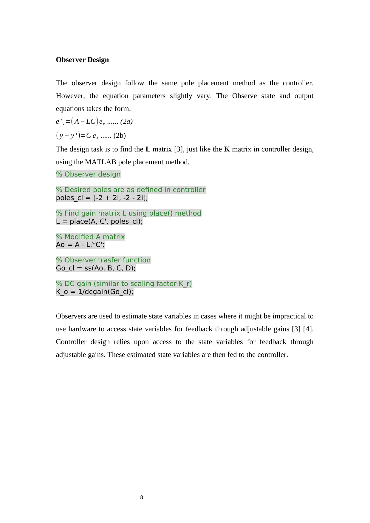
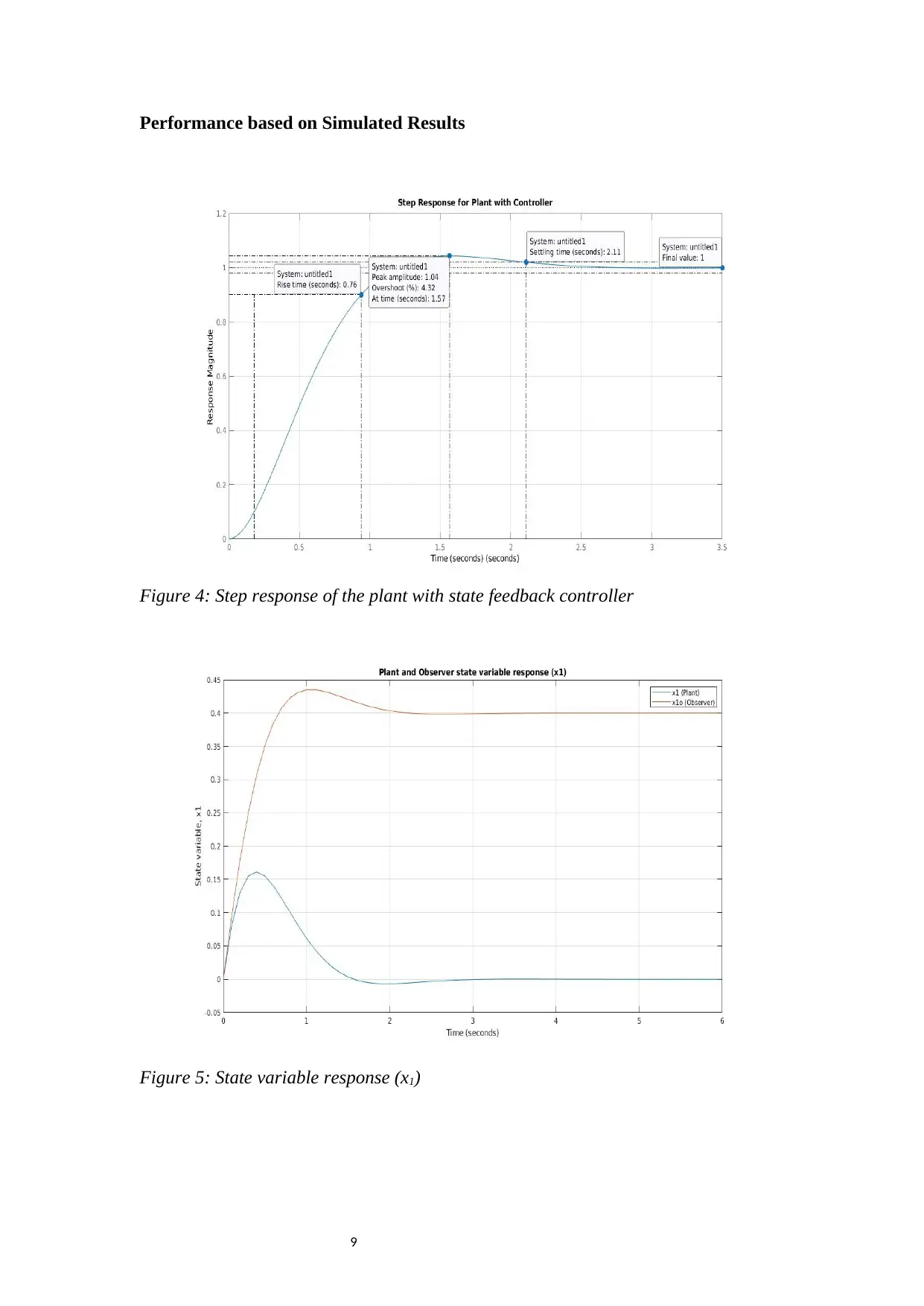
This project report details the design and analysis of a control system, focusing on a second-order plant represented by a transfer function. The report begins with an overview of the plant, including its transfer function and its application as a mass-spring-damper system, with equivalent control systems block diagrams. The project then investigates the plant's performance, examining its stability, observability, and controllability using MATLAB. The subsequent sections focus on designing a state feedback controller and an observer using pole-placement techniques to improve the system's response characteristics, specifically reducing overshoot and settling time. The design process includes simulating the system in MATLAB and analyzing the step response. The results demonstrate the effectiveness of the designed controller and observer in enhancing the plant's performance. The project also highlights the importance of simulation in engineering designs, showcasing how it provides valuable insights and allows for performance optimization before hardware implementation. The report concludes with a bibliography of relevant sources.

i
CONTROL SYSTEMS DESIGN
{{ Student Details here }}

ii
Table of Contents
Practical engineering plant.............................................................................................3
Equivalent control systems block diagrams...................................................................3
Plant Performance..........................................................................................................4
Stability...................................................................................................................4
Observability...........................................................................................................6
Controllability.........................................................................................................6
Unit Step Time Response........................................................................................7
State Feedback Controller Design..................................................................................8
Observer Design...........................................................................................................10
Performance based on Simulated Results....................................................................11
Importance of Simulation in Engineering Designs......................................................13
Bibliography.................................................................................................................14
List of Figures
Figure 1 : Output Feedback Block Diagram.....................................................................3
Figure 2 : State Feedback Block Diagram........................................................................4
Figure 3 : Plant's Step Response.......................................................................................8
Figure 4 : Step response of the plant with state feedback controller..............................11
Figure 5 : State variable response (x1)............................................................................11
Figure 6 : State variable response (x2)............................................................................12
Figure 7 : Controlled Plant and Observer response.......................................................12

1
Practical engineering plant
The system plant given has the following transfer function:
C (s)
U ( s) =Gp (s )= 4
s2+ 0.8 s+ 4 ...... (1a)
This is second order system transfer function which takes the general form of:
C (s)
U ( s) =Gp (s )= ω2
s2+2 ξωs +ω2 ...... (1b)
This system form is commonly known as mass-spring-damper (MKS) system [1].
Such a system find applications in designing the car suspension systems in
mechanical engineering and relay switching in electrical engineering. It is also a
useful concept in multidisciplinary robotics and aeronautics systems [8].
A car suspension system consists of of tires, tire air, springs, shock absorbers and
linkages. These components are connected such that a vehicle is allowed a relative
motion between the two [9].
Equivalent control systems block diagrams
Figure 1: Output Feedback Block Diagram

2
Figure 2: State Feedback Block Diagram
Figures 1 and 2 show output and state feedback block diagrams respectively. The two
blocks are similar in that both use feedback mechanism and contains a controller.
However, they differ both in the feedback method and controller implementation. The
output feedback block diagram in Figure 1 compares the reference signal with the
system output (assuming unity feedback path: H(s) = 1) to get the control error. A
controller is developed which takes the error as input and generates an input signal to
the plant with the goal of deriving the error to zero [6]. For state feedback block
diagram in Figure 2, every state variable (X) is fed back through a gain matrix K. The
result is subtracted from a scaled reference signal (due to Kr factor) and fed directly
into the plant. In this case, both Kr, summing junction and gain matrix form the
controller [2]. The gain matrix K is used to attain stability while the scaling factor Kr
is used to maintain acceptable steady-state error performance [7].
Plant Performance
Stability
A control system is table if and only if all its poles lied in the left half plane (LHP) of
a complex plane [1]. In state-space domain, the poles of the system (plant) are the
eigen values of the A matrix [2]. To get the state-space representation of the transfer
function given in equation (1a), we MATLAB’s tf2ss() function is used [8]. The
MATLAB code snippet used for this task is shown below:

3
% Define the transfer function numerator and denominator
num = [0 0 4];
den = [1 0.8 4];
% Get A, B, C and D parameters from the transfer function
[A, B, C, D] = tf2ss(num, den);
Results:
A =
-0.8000 -4.0000
1.0000 0
B =
1
0
C =
0 4
D =
0
Plant’s poles:
% System (plant) poles
p = eig(A);
p =
-0.4000 + 1.9596i
-0.4000 - 1.9596i
The plant has poles at -0.4 + 1.9506i and -0.4 - 1.9596i. These two poles lies
on the left hand of the complex plane, hence the system is stable.
Observability
A system is said to be observable if it is possible to determine the initial states of the
system by observing outputs in finite time duration [1]. This is however best done or
defined from mathematical concepts. To do so, Kalman's test is used.
The Kalman's test involves two steps: define the observability matrix, Qo and then

4
find the determinant of this matrix. If the determinant is not equal to zero, then the
system is observable [6] [4].
Qo is defines as: Qo = [CT ATCT (AT)2CT ... (AT)n-1CT], Where A and C are state-
space parameters and n is the order of the n×n A matrix. In this case, n = 2. Hence,
Qo = [CT ATCT].
Solving for [CT ATCT] in MATLAB, we have:
% Calculate M_o and its determinant
CT = C';
ATCT = A' * C';
M_o = [CT ATCT];
det_Mo = det(M_o);
CT =
0
4
ATCT =
4
0
M_o =
0 4
4 0
det_Mo =
-16
The determinant of Qo = -16 != 0. Hence, the plant system is observable.
Controllability
A system is said to be controllable if it is possible to change the initial states of the
system to some other desired states by a controlled input in a finite time duration [1].
Just like in observability, controllability can as well be defined from mathematical
concepts using another form of Kalman's test.
The Kalman's test in controllability also involves two steps: define the controllability
matrix, Qc and then find the determinant of this matrix. If the determinant is not
equal to zero, then the system is controllable [6].
Qc is defines as: Qc = [B AB A2B ... An-1B], Where A and B are state-space parameters
and n is the order of the n×n A matrix. In this case, n = 2. Hence,
Qc = [A AB].
Solving for [A AB] in MATLAB, we have:
% Calculate M_c and its detrminant

5
AB = A * B;
M_c = [B AB];
det_Mc = det(M_c);
A =
-0.8000 -4.0000
1.0000 0
AB =
-0.8000
1.0000
M_c =
1.0000 -0.8000
0 1.0000
det_Mc =
1
The determinant of Qc = 1 != 0. Hence, the plant system is controllable.
Unit Step Time Response
The MATLAB step() function is used to simulate the plant’s transfer function.
% Getthe plant's transfer function
Gp = ss(A, B, C, D);
% Plant's step response
figure(1)
step(Gp), grid;

6
Figure 3: Plant's Step Response
The step response shows that the system is stable. Despite having a over 50%
overshoot (52.7%), the plant system finally settles at 1 which translates in zero
steady-state error. The system however takes a considerable amount of time (9.8
seconds) to settle. The overshoot and settling time are the two candidates for
consideration during the controller design since they require improvement.
State Feedback Controller Design
This section deals with the design of state feedback controller. The controller design
will be influenced by the need to reduce the system overshoot (52.7%) and settling
time (9.8 seconds) which were marked as undesirable from Figure 3. Precisely, a
controller is designed to achieve less than 10% overshoot and less than 5 seconds rise
time.
To achieve this, pole-placement method is used in the controller design. In reference
to Figure 2, pole placement involves finding the gain matrix K to achieve the desired
performance and then solve for the appropriate value of the scaling factor Kr to ensure
the desired steady-state response [5]. The whole process involves finding the desired
poles should be placed. In this case, the real parts of the poles (0.4) are almost five

7
times less compared to the imaginary parts (1.9596). This is the main cause of
overshoot. Making the two parts equal or close will reduce the overshoot. There is an
option of either reducing the imaginary part to 0.4, increasing the real part to 1.9596,
or using different values altogether. Each choice however comes with a consequence.
For instance, lowering the imaginary part to 0.4 results in high settling time which
may not be desirable [7]. Again, pulling the poles very far to the left might require
more power than the system can provide to give the desired response [6]. With this in
mind, the poles are placed at -2 + 2i and -2 - 2i points. The gain matrix K is
calculated using the MATLAB place() method.
% Define the desired poles
poles_cl = [-2 + 2i, -2 - 2i];
% Find gain matrix K using place() method
K = place(A, B, poles_cl);
% Compute the new closed-loop transfer function
Gp_cl = ss(A-B*K, B, C, D);
% Find the dynamic scaling factor Kr
K_r = 1/dcgain(Gp_cl);

8
Observer Design
The observer design follow the same pole placement method as the controller.
However, the equation parameters slightly vary. The Observe state and output
equations takes the form:
e 'x =( A − LC)ex ...... (2a)
( y − y ' )=C ex ...... (2b)
The design task is to find the L matrix [3], just like the K matrix in controller design,
using the MATLAB pole placement method.
% Observer design
% Desired poles are as defined in controller
poles_cl = [-2 + 2i, -2 - 2i];
% Find gain matrix L using place() method
L = place(A, C', poles_cl);
% Modified A matrix
Ao = A - L.*C';
% Observer trasfer function
Go_cl = ss(Ao, B, C, D);
% DC gain (similar to scaling factor K_r)
K_o = 1/dcgain(Go_cl);
Observers are used to estimate state variables in cases where it might be impractical to
use hardware to access state variables for feedback through adjustable gains [3] [4].
Controller design relies upon access to the state variables for feedback through
adjustable gains. These estimated state variables are then fed to the controller.

9
Performance based on Simulated Results
Figure 4: Step response of the plant with state feedback controller
Figure 5: State variable response (x1)

10
Figure 6: State variable response (x2)
Figure 7: Controlled Plant and Observer response