Interest Rate Risk: Short-Term vs Long-Term Bonds

The assignment content discusses bond values and interest rate risk. It provides examples of bonds selling at a premium and discount, using TVM templates to calculate the bond values. The content also illustrates how shorter-term bonds are less affected by changes in market rates compared to longer-term bonds.

Corporate Finance
Phantom Student
1

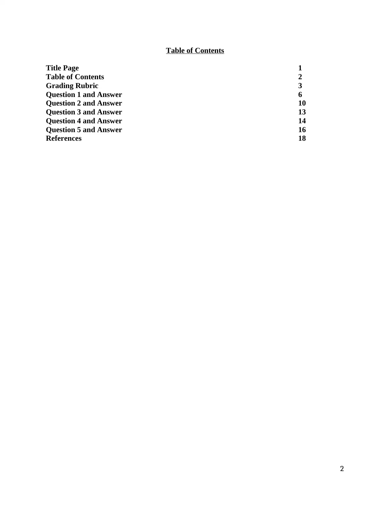
Table of Contents
Title Page 1
Table of Contents 2
Grading Rubric 3
Question 1 and Answer 6
Question 2 and Answer 10
Question 3 and Answer 13
Question 4 and Answer 14
Question 5 and Answer 16
References 18
2

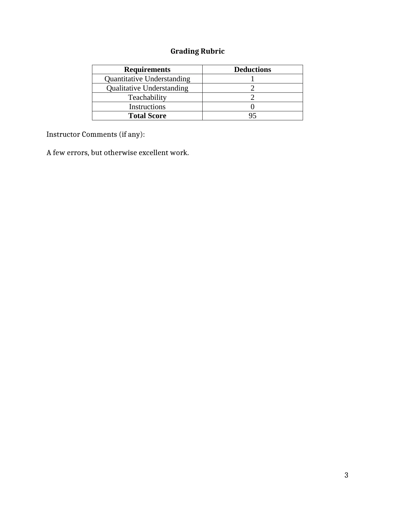
Grading Rubric
Requirements Deductions
Quantitative Understanding 1
Qualitative Understanding 2
Teachability 2
Instructions 0
Total Score 95
Instructor Comments (if any):
A few errors, but otherwise excellent work.
3

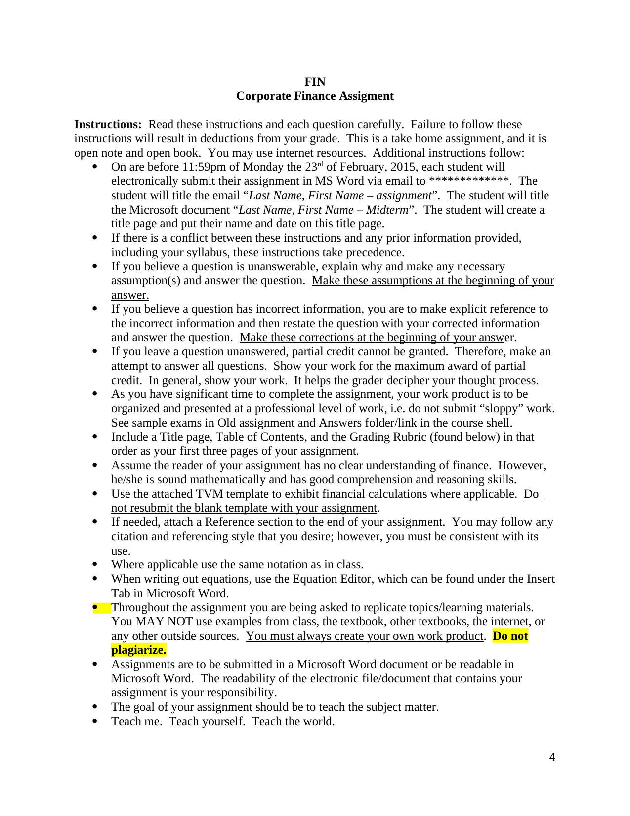
FIN
Corporate Finance Assigment
Instructions: Read these instructions and each question carefully. Failure to follow these
instructions will result in deductions from your grade. This is a take home assignment, and it is
open note and open book. You may use internet resources. Additional instructions follow:
 On are before 11:59pm of Monday the 23rd of February, 2015, each student will
electronically submit their assignment in MS Word via email to *************. The
student will title the email “Last Name, First Name – assignment”. The student will title
the Microsoft document “Last Name, First Name – Midterm”. The student will create a
title page and put their name and date on this title page.
 If there is a conflict between these instructions and any prior information provided,
including your syllabus, these instructions take precedence.
 If you believe a question is unanswerable, explain why and make any necessary
assumption(s) and answer the question. Make these assumptions at the beginning of your
answer.
 If you believe a question has incorrect information, you are to make explicit reference to
the incorrect information and then restate the question with your corrected information
and answer the question. Make these corrections at the beginning of your answer.
 If you leave a question unanswered, partial credit cannot be granted. Therefore, make an
attempt to answer all questions. Show your work for the maximum award of partial
credit. In general, show your work. It helps the grader decipher your thought process.
 As you have significant time to complete the assignment, your work product is to be
organized and presented at a professional level of work, i.e. do not submit “sloppy” work.
See sample exams in Old assignment and Answers folder/link in the course shell.
 Include a Title page, Table of Contents, and the Grading Rubric (found below) in that
order as your first three pages of your assignment.
 Assume the reader of your assignment has no clear understanding of finance. However,
he/she is sound mathematically and has good comprehension and reasoning skills.
 Use the attached TVM template to exhibit financial calculations where applicable. Do
not resubmit the blank template with your assignment.
 If needed, attach a Reference section to the end of your assignment. You may follow any
citation and referencing style that you desire; however, you must be consistent with its
use.
 Where applicable use the same notation as in class.
 When writing out equations, use the Equation Editor, which can be found under the Insert
Tab in Microsoft Word.
 Throughout the assignment you are being asked to replicate topics/learning materials.
You MAY NOT use examples from class, the textbook, other textbooks, the internet, or
any other outside sources. You must always create your own work product. Do not
plagiarize.
 Assignments are to be submitted in a Microsoft Word document or be readable in
Microsoft Word. The readability of the electronic file/document that contains your
assignment is your responsibility.
 The goal of your assignment should be to teach the subject matter.
 Teach me. Teach yourself. Teach the world.
4

Have fun and good luck.
5

Question 1: Assume that a public corporation has 3,000,000 shares outstanding. First, you are to
create the necessary Balance Sheets and Income Statements and then calculate the annual Cash
Flow from Assets (aka: CFFA or Free Cash Flows (FCF)) for this corporation. A constraint here
is that your CFFA must range between $6,000,000 and $10,000,000 annually. Second, after
calculating CFFA, you are to assume that this corporation is a no-growth perpetuity and estimate
its present value (aka: intrinsic value). Assume the market determined risk adjusted required rate
of return is 6.125% for this corporation. Said another way, you are to replicate and explain the
relevant parts of the textbook, notes, and lectures associated with CFFA and intrinsic value of the
firm estimations. Teach me the concepts.
Answer 1: Part 1: Calculating annual Cash Flow from Assets
Notice, that as this question is written, it is unanswerable. Specifically, no marginal tax rate (τ)
is provided making it impossible to estimate Net Income (and other necessary calculations).
Accordingly, let the marginal tax rate equal 55% for this firm.
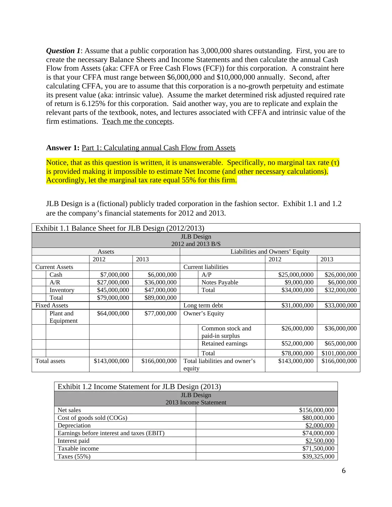
JLB Design is a (fictional) publicly traded corporation in the fashion sector. Exhibit 1.1 and 1.2
are the company’s financial statements for 2012 and 2013.
Exhibit 1.1 Balance Sheet for JLB Design (2012/2013)
JLB Design
2012 and 2013 B/S
Assets Liabilities and Owners’ Equity
2012 2013 2012 2013
Current Assets Current liabilities
Cash $7,000,000 $6,000,000 A/P $25,000,0000 $26,000,000
A/R $27,000,000 $36,000,000 Notes Payable $9,000,000 $6,000,000
Inventory $45,000,000 $47,000,000 Total $34,000,000 $32,000,000
Total $79,000,000 $89,000,000
Fixed Assets Long term debt $31,000,000 $33,000,000
Plant and
Equipment
$64,000,000 $77,000,000 Owner’s Equity
Common stock and
paid-in surplus
$26,000,000 $36,000,000
Retained earnings $52,000,000 $65,000,000
Total $78,000,000 $101,000,000
Total assets $143,000,000 $166,000,000 Total liabilities and owner’s
equity
$143,000,000 $166,000,000
Exhibit 1.2 Income Statement for JLB Design (2013)
JLB Design
2013 Income Statement
Net sales $156,000,000
Cost of goods sold (COGs) $80,000,000
Depreciation $2,000,000
Earnings before interest and taxes (EBIT) $74,000,000
Interest paid $2,500,000
Taxable income $71,500,000
Taxes (55%) $39,325,000
6

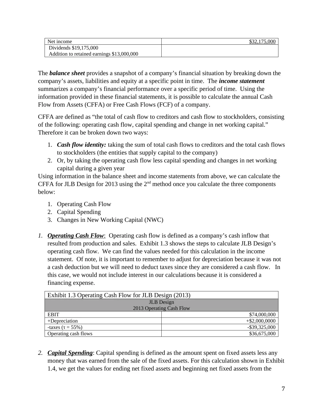
Net income $32,175,000
Dividends $19,175,000
Addition to retained earnings $13,000,000
The balance sheet provides a snapshot of a company’s financial situation by breaking down the
company’s assets, liabilities and equity at a specific point in time. The income statement
summarizes a company’s financial performance over a specific period of time. Using the
information provided in these financial statements, it is possible to calculate the annual Cash
Flow from Assets (CFFA) or Free Cash Flows (FCF) of a company.
CFFA are defined as “the total of cash flow to creditors and cash flow to stockholders, consisting
of the following: operating cash flow, capital spending and change in net working capital.”
Therefore it can be broken down two ways:
1. Cash flow identity: taking the sum of total cash flows to creditors and the total cash flows
to stockholders (the entities that supply capital to the company)
2. Or, by taking the operating cash flow less capital spending and changes in net working
capital during a given year
Using information in the balance sheet and income statements from above, we can calculate the
CFFA for JLB Design for 2013 using the 2nd method once you calculate the three components
below:
1. Operating Cash Flow
2. Capital Spending
3. Changes in New Working Capital (NWC)
1. Operating Cash Flow: Operating cash flow is defined as a company’s cash inflow that
resulted from production and sales. Exhibit 1.3 shows the steps to calculate JLB Design’s
operating cash flow. We can find the values needed for this calculation in the income
statement. Of note, it is important to remember to adjust for depreciation because it was not
a cash deduction but we will need to deduct taxes since they are considered a cash flow. In
this case, we would not include interest in our calculations because it is considered a
financing expense.
Exhibit 1.3 Operating Cash Flow for JLB Design (2013)
JLB Design
2013 Operating Cash Flow
EBIT $74,000,000
+Depreciation +$2,000,0000
-taxes (τ = 55%) -$39,325,000
Operating cash flows $36,675,000
2. Capital Spending: Capital spending is defined as the amount spent on fixed assets less any
money that was earned from the sale of the fixed assets. For this calculation shown in Exhibit
1.4, we get the values for ending net fixed assets and beginning net fixed assets from the
7

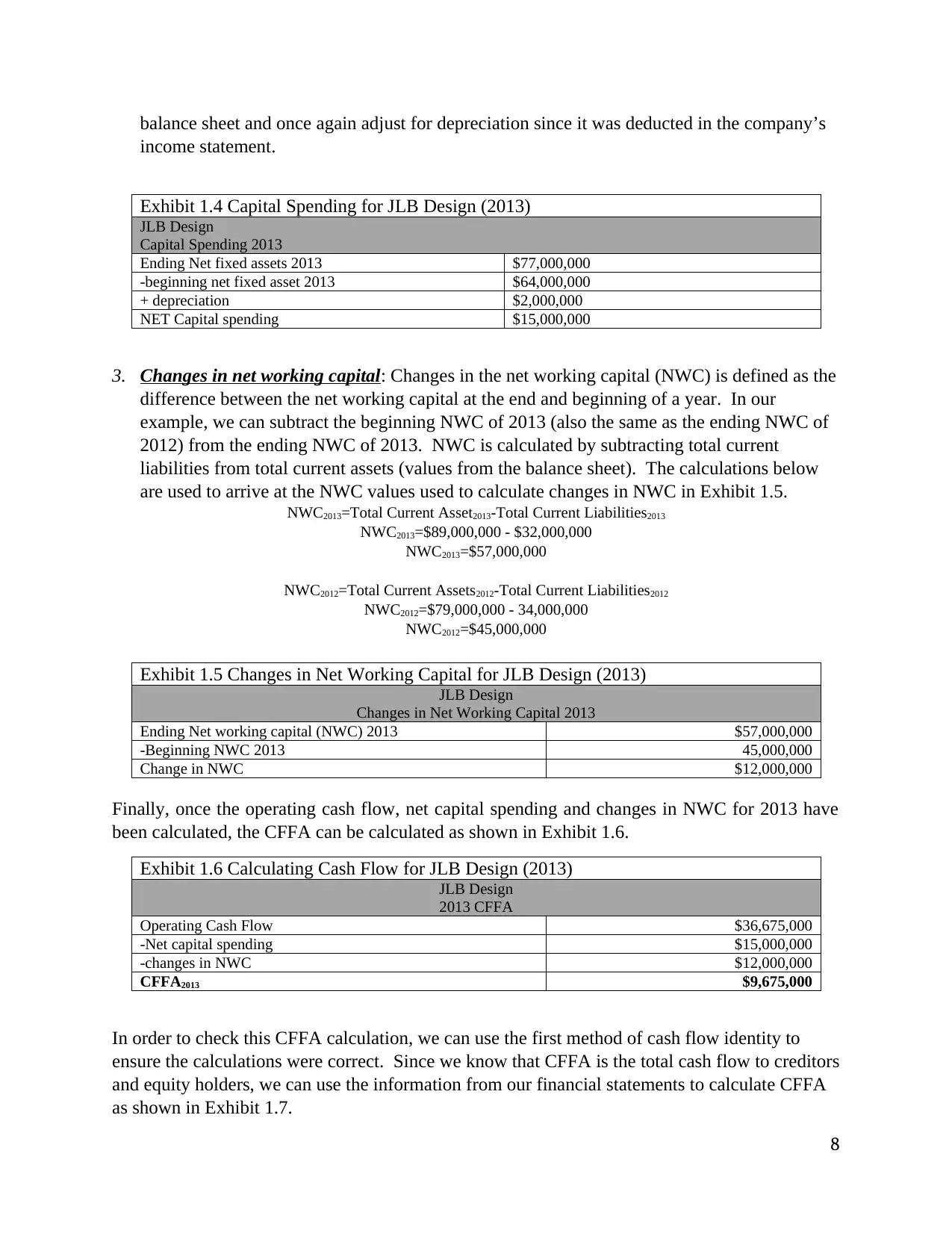
balance sheet and once again adjust for depreciation since it was deducted in the company’s
income statement.
Exhibit 1.4 Capital Spending for JLB Design (2013)
JLB Design
Capital Spending 2013
Ending Net fixed assets 2013 $77,000,000
-beginning net fixed asset 2013 $64,000,000
+ depreciation $2,000,000
NET Capital spending $15,000,000
3. Changes in net working capital: Changes in the net working capital (NWC) is defined as the
difference between the net working capital at the end and beginning of a year. In our
example, we can subtract the beginning NWC of 2013 (also the same as the ending NWC of
2012) from the ending NWC of 2013. NWC is calculated by subtracting total current
liabilities from total current assets (values from the balance sheet). The calculations below
are used to arrive at the NWC values used to calculate changes in NWC in Exhibit 1.5.
NWC2013=Total Current Asset2013-Total Current Liabilities2013
NWC2013=$89,000,000 - $32,000,000
NWC2013=$57,000,000
NWC2012=Total Current Assets2012-Total Current Liabilities2012
NWC2012=$79,000,000 - 34,000,000
NWC2012=$45,000,000
Exhibit 1.5 Changes in Net Working Capital for JLB Design (2013)
JLB Design
Changes in Net Working Capital 2013
Ending Net working capital (NWC) 2013 $57,000,000
-Beginning NWC 2013 45,000,000
Change in NWC $12,000,000
Finally, once the operating cash flow, net capital spending and changes in NWC for 2013 have
been calculated, the CFFA can be calculated as shown in Exhibit 1.6.
Exhibit 1.6 Calculating Cash Flow for JLB Design (2013)
JLB Design
2013 CFFA
Operating Cash Flow $36,675,000
-Net capital spending $15,000,000
-changes in NWC $12,000,000
CFFA2013 $9,675,000
In order to check this CFFA calculation, we can use the first method of cash flow identity to
ensure the calculations were correct. Since we know that CFFA is the total cash flow to creditors
and equity holders, we can use the information from our financial statements to calculate CFFA
as shown in Exhibit 1.7.
8

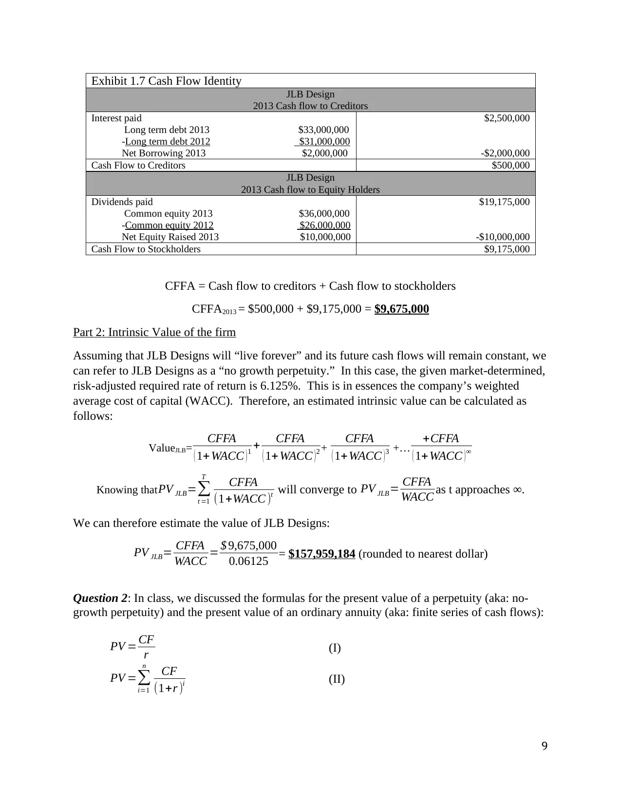
Exhibit 1.7 Cash Flow Identity
JLB Design
2013 Cash flow to Creditors
Interest paid
Long term debt 2013 $33,000,000
-Long term debt 2012 $31,000,000
Net Borrowing 2013 $2,000,000
$2,500,000
-$2,000,000
Cash Flow to Creditors $500,000
JLB Design
2013 Cash flow to Equity Holders
Dividends paid
Common equity 2013 $36,000,000
-Common equity 2012 $26,000,000
Net Equity Raised 2013 $10,000,000
$19,175,000
-$10,000,000
Cash Flow to Stockholders $9,175,000
CFFA = Cash flow to creditors + Cash flow to stockholders
CFFA2013 = $500,000 + $9,175,000 = $9,675,000
Part 2: Intrinsic Value of the firm
Assuming that JLB Designs will “live forever” and its future cash flows will remain constant, we
can refer to JLB Designs as a “no growth perpetuity.” In this case, the given market-determined,
risk-adjusted required rate of return is 6.125%. This is in essences the company’s weighted
average cost of capital (WACC). Therefore, an estimated intrinsic value can be calculated as
follows:
ValueJLB= CFFA
( 1+WACC )1 + CFFA
( 1+ WACC )2 + CFFA
( 1+WACC )3 +… +CFFA
( 1+WACC )∞
Knowing thatPV JLB=∑
t =1
T CFFA
(1+WACC )t will converge to PV JLB= CFFA
WACC as t approaches ∞.
We can therefore estimate the value of JLB Designs:
PV JLB= CFFA
WACC = $ 9,675,000
0.06125 = $157,959,184 (rounded to nearest dollar)
Question 2: In class, we discussed the formulas for the present value of a perpetuity (aka: no-
growth perpetuity) and the present value of an ordinary annuity (aka: finite series of cash flows):
PV = CF
r (I)
PV =∑
i=1
n CF
(1+r )i (II)
9

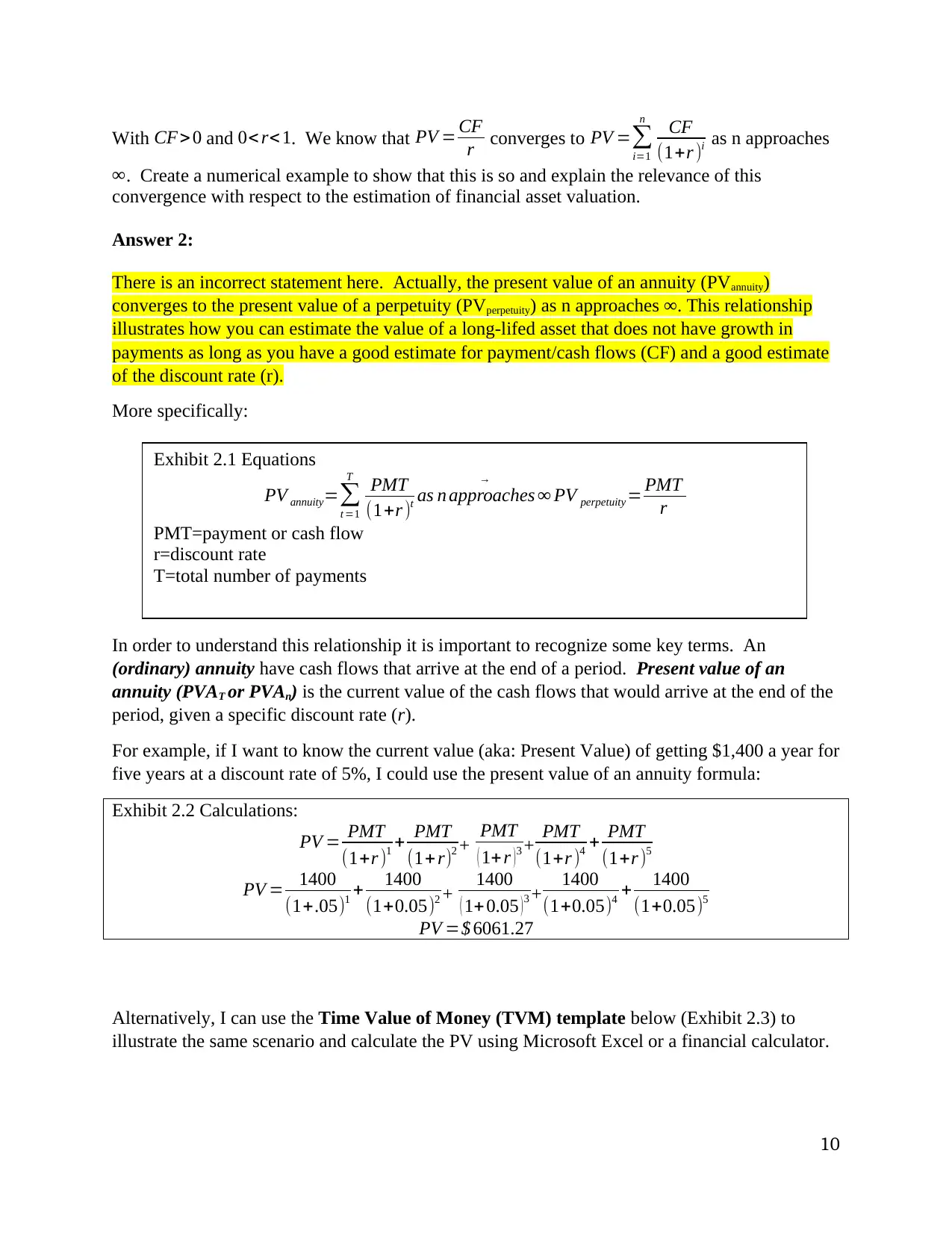
With CF> 0 and 0< r< 1. We know that PV = CF
r converges to PV =∑
i=1
n CF
(1+r )i as n approaches
∞. Create a numerical example to show that this is so and explain the relevance of this
convergence with respect to the estimation of financial asset valuation.
Answer 2:
There is an incorrect statement here. Actually, the present value of an annuity (PVannuity)
converges to the present value of a perpetuity (PVperpetuity) as n approaches ∞. This relationship
illustrates how you can estimate the value of a long-lifed asset that does not have growth in
payments as long as you have a good estimate for payment/cash flows (CF) and a good estimate
of the discount rate (r).
More specifically:
In order to understand this relationship it is important to recognize some key terms. An
(ordinary) annuity have cash flows that arrive at the end of a period. Present value of an
annuity (PVAT or PVAn) is the current value of the cash flows that would arrive at the end of the
period, given a specific discount rate (r).
For example, if I want to know the current value (aka: Present Value) of getting $1,400 a year for
five years at a discount rate of 5%, I could use the present value of an annuity formula:
Exhibit 2.2 Calculations:
PV = PMT
(1+r )1 + PMT
(1+ r)2 + PMT
( 1+r )3 + PMT
(1+r )4 + PMT
(1+r )5
PV = 1400
(1+.05)1 + 1400
(1+0.05)2 + 1400
( 1+ 0.05 ) 3 + 1400
(1+0.05)4 + 1400
(1+0.05)5
PV =$ 6061.27
Alternatively, I can use the Time Value of Money (TVM) template below (Exhibit 2.3) to
illustrate the same scenario and calculate the PV using Microsoft Excel or a financial calculator.
10
Exhibit 2.1 Equations
PV annuity=∑
t =1
T PMT
(1+r )t as n approaches ∞
→
PV perpetuity = PMT
r
PMT=payment or cash flow
r=discount rate
T=total number of payments

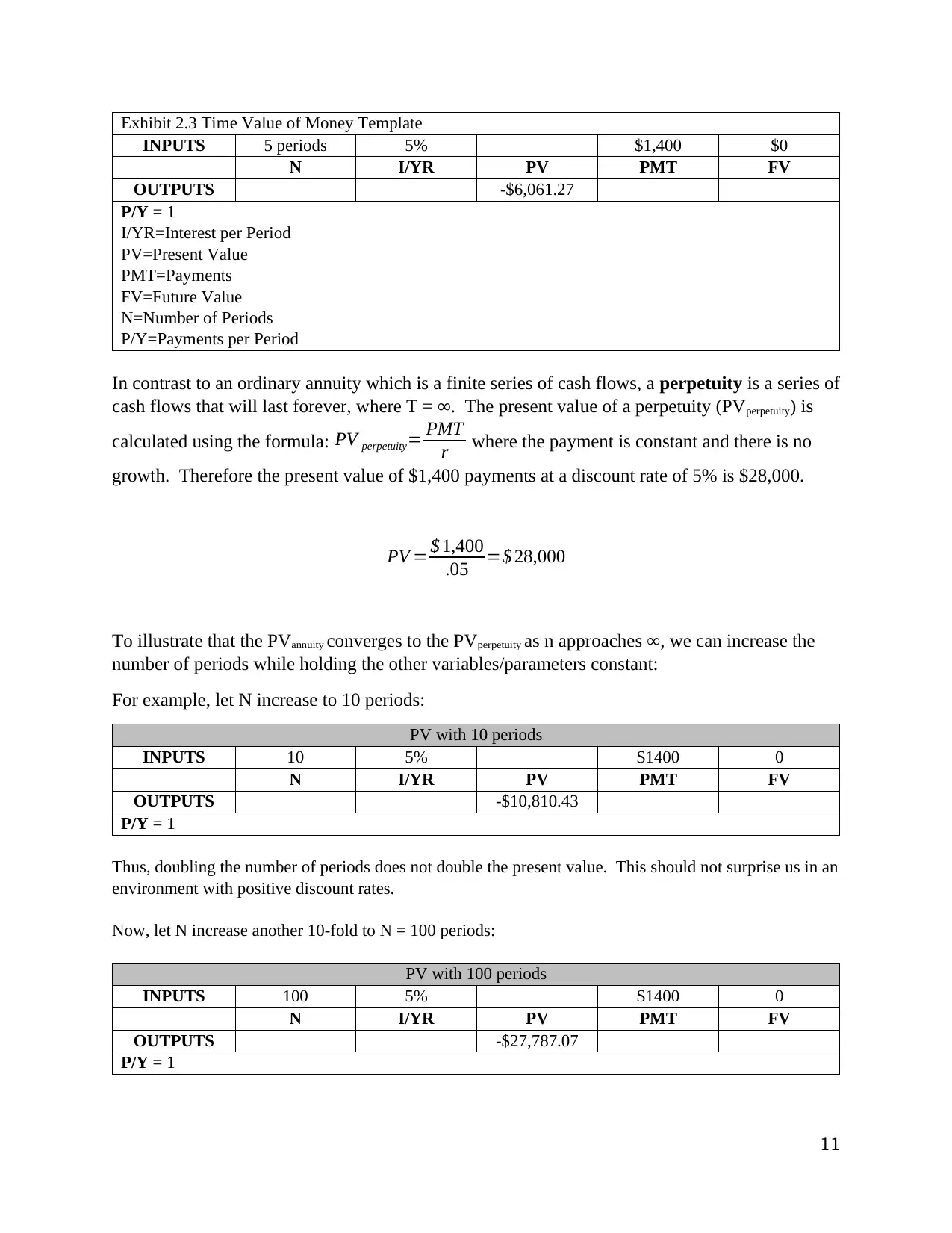
Exhibit 2.3 Time Value of Money Template
INPUTS 5 periods 5% $1,400 $0
N I/YR PV PMT FV
OUTPUTS -$6,061.27
P/Y = 1
I/YR=Interest per Period
PV=Present Value
PMT=Payments
FV=Future Value
N=Number of Periods
P/Y=Payments per Period
In contrast to an ordinary annuity which is a finite series of cash flows, a perpetuity is a series of
cash flows that will last forever, where T = ∞. The present value of a perpetuity (PVperpetuity) is
calculated using the formula: PV perpetuity= PMT
r where the payment is constant and there is no
growth. Therefore the present value of $1,400 payments at a discount rate of 5% is $28,000.
PV = $ 1,400
.05 =$ 28,000
To illustrate that the PVannuity converges to the PVperpetuity as n approaches ∞, we can increase the
number of periods while holding the other variables/parameters constant:
For example, let N increase to 10 periods:
PV with 10 periods
INPUTS 10 5% $1400 0
N I/YR PV PMT FV
OUTPUTS -$10,810.43
P/Y = 1
Thus, doubling the number of periods does not double the present value. This should not surprise us in an
environment with positive discount rates.
Now, let N increase another 10-fold to N = 100 periods:
PV with 100 periods
INPUTS 100 5% $1400 0
N I/YR PV PMT FV
OUTPUTS -$27,787.07
P/Y = 1
11

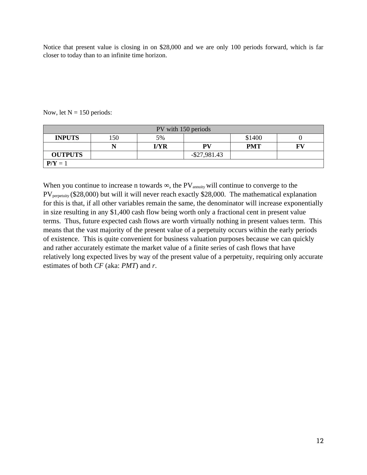
Notice that present value is closing in on $28,000 and we are only 100 periods forward, which is far
closer to today than to an infinite time horizon.
Now, let N = 150 periods:
PV with 150 periods
INPUTS 150 5% $1400 0
N I/YR PV PMT FV
OUTPUTS -$27,981.43
P/Y = 1
When you continue to increase n towards ∞, the PVannuity will continue to converge to the
PVperpetuity ($28,000) but will it will never reach exactly $28,000. The mathematical explanation
for this is that, if all other variables remain the same, the denominator will increase exponentially
in size resulting in any $1,400 cash flow being worth only a fractional cent in present value
terms. Thus, future expected cash flows are worth virtually nothing in present values term. This
means that the vast majority of the present value of a perpetuity occurs within the early periods
of existence. This is quite convenient for business valuation purposes because we can quickly
and rather accurately estimate the market value of a finite series of cash flows that have
relatively long expected lives by way of the present value of a perpetuity, requiring only accurate
estimates of both CF (aka: PMT) and r.
12

Question 3: Consider PV =∑
i=1
n CF
(1+r )i which expands to PV = CF
(1+r )1 + CF
(1+ r)2 +…+ CF
(1+r )n
In terms of present value (PV), what happens to the right hand side of the equation as r
approaches zero (0)?
Answer 3:
When calculating present value (PV), r represents the discount rate. As r approaches zero, the
denominator of the present value formula approaches one. Therefore, as r approaches zero, the
sum of the future expected cash flows get continually closer to PV.
Expressed in equation form, if PV =∑
i=1
n CF
(1+r )i and r =0, thenPV =∑
i=1
n
CF.
13

Question 4: Considering interest changes and bond prices, develop an example to explain how a
bond selling at a premium arises and how a bond selling at a discount arises. Use the relevant
parts of the textbook, notes, and lectures to teach me the concept.
Answer 4:
First, for the example of a bond selling at a premium, we will use a 7 year, semiannually
compounded bond with a par value of $5,000 and a coupon rate of 8% per period or 16%
annually. At issuance, assuming the market rate equals the coupon rate, which is most common.
V B =$ 400 [ 1
.08 − 1
.08 ( 1+.08 )14 ]+ $ 5,000
( 1+.08 )14
This can be shown by way of a Time Value of Money template as well:
INPUTS 14 periods 8% $400 $5,000
N I/P PV PMT FV
OUTPUT $5,000
P/Y = 1
Now suppose we have moved forward 3 years and the market interest rate has fallen to 5% per
period ( rd =10 % annually).
V B =$ 400 [ 1
.05 − 1
.05 ( 1+.05 ) 8 ] + $ 5,000
( 1+ .05 ) 8
Again, using a TVM template:
INPUTS 8 periods 5% $400 $5,000
N I/P PV PMT FV
OUTPUT $5,969.48
P/Y = 1
This bond is said to be selling at a premium. It is offering an interest payment of 8% per period
of its par value. New bonds, issued at this point in time, will only pay 5% per period of their par
value. Therefore, investors are willing to pay a premium to acquire this asset because it is
offering a rate of return that is higher than the market is currently offering (8% per period vs 5%
per period) on comparable bonds.
Second, let’s look at an example of a bond selling at a discount. For the discount bond example,
we will use a 20 year, annually compounded bond with a par value of $8,500 and a coupon rate
of 3.2%. At issuance, assuming the market rate equals the coupon rate, which is most common:
14

V B =$ 272 [ 1
.032 − 1
.032 ( 1+.032 )20 ]+ $ 8,500
( 1+.032 )20
Again, using a TVM template:
INPUTS 20 periods 3.2% $272 $8,500
N I/P PV PMT FV
OUTPUT $8,500
P/Y = 1
Now suppose we have moved forward 14 years, and the market interest rate ( rd ) has risen to
7.5%. Now,
V B =$ 272 [ 1
.075 − 1
.075 ( 1+.075 ) 6 ] + $ 8,500
( 1+.075 ) 6
INPUTS 6 periods 7.5% $272 $8,500
N I/P PV PMT FV
OUTPUT $6,784.40
P/Y = 1
This bond is said to be selling at a discount. Investors can purchase newly issued bonds of
comparable risk paying interest of 7.5% of their par value. Why would an investor want to only
earn 3.2%? In order to sell this bond under the current market conditions, the bond holder must
offer a discount and sell the bond at less than its face value in order to move the security. Said
another way, this bond with its 3.2% coupon is priced to yield 7.5% at $6,784.40.
15

Question 5: Develop an explain interest rate risk. Basically, you are to replicate and
explain the relevant parts of your textbook, notes, and lectures. Make sure that you
highlight the fact that shorter-term bonds have more interest rate sensitivity than longer-term
bonds. Teach me the concept
There is an incorrect statement here. Specifically, shorter-term bonds are not more sensitive to
interest rate risk than longer-term bonds. In fact, it is longer-term bonds that suffer more than
shorter-term bonds to interest rate risk exposure.
Interest rate risk is the risk of bond value changes associated with fluctuations in the market-
determined, risk-adjusted required rate of return (rd). Bonds with varying maturity lengths
have different sensitivities to fluctuations in the market interest rate. Shorter-term bonds, or
bonds closer to maturity, are less sensitive to interest rate changes and as a result they are said to
suffer less interest rate sensitivity. Conversely, longer-term bonds have a greater interest rate
risks and are greatly affected by changes in the market rate.
Suppose you have two 10% coupon bonds, one with a maturity of 1 year and the other with a
maturity of 25 years. All else equal, the 1-year bond will be less sensitive to changes in the
market rate than the 25-year bond. Each bond is annually compounded and its par value is
$1,500. Exhibit 5.1a and 5.1b illustrate this phenomenon graphically and plots the changes that
occur to bond value when the market rate is changed from 10% to 5% and 15% and 20%. At a
10% market rate, rd=rc and par value of the bond is $1500 as expected. The steepness of the
slopes of the graphs show how the shorter-term bond does not change in value as much as the
longer-term bond when the market rate changes.
Exhibit 5.2 shows the TVM templates used to calculate the bond value for the 1-year bond in
comparison to a 25-year bond.
Exhibit 5.1a Interest Rate Risk and Time to Maturity
Interest Rate 1 year bond 25 year bond
5% $1,571.43 $2,557.05
10% $1,500.00 $1,500.00
15% $1,434.78 $1,015.19
20% $1,375.00 $757.86
16

0% 5% 10% 15% 20%
$0.00
$500.00
$1,000.00
$1,500.00
$2,000.00
$2,500.00
$3,000.00
$2,557.05
$1,500.00
$1,015.19 $757.86
$1,571.43 $1,434.78 $1,375.00
Exhibit 5.1b Interest Rate Risk and Time to Maturity
1 year bond 25 year bond
The TVM Templates below indicate the calculations used to calculate the bond values with a
10% coupon rate with fluctuating interest rates for a 1-year bond versus a 25-year bond.
Exhibit 5.2: TVM Templates used to illustrate Interest Rate Risk
5% interest, 1-year bond
INPUTS 1 5% +$150 $1500
N I/YR PV PMT FV
OUTPUTS -$1,571.43
1/Y=1
10% interest, 1-year bond
INPUTS 1 10% +$150 $1500
N I/YR PV PMT FV
OUTPUTS -$1500.00
1/Y=1
15% interest, 1-year bond
INPUTS 1 15% +$150 $1500
N I/YR PV PMT FV
OUTPUTS -$1,434.78
1/Y=1
20% interest, 1-year bond
INPUTS 1 20% +$150 $1500
N I/YR PV PMT FV
OUTPUTS -$1,375.00
1/Y=1
17

5% interest, 25-year bond
INPUTS 25 5% +$150 $1500
N I/YR PV PMT FV
OUTPUTS -$2,557.05
1/Y=1
10% interest, 25-year bond
INPUTS 25 10% +$150 $1500
N I/YR PV PMT FV
OUTPUTS -$1500.00
1/Y=1
15% interest, 25-year bond
INPUTS 25 15% +$150 $1500
N I/YR PV PMT FV
OUTPUTS -$1,015.19
1/Y=1
20% interest, 25-year bond
INPUTS 25 20% +$150 $1500
N I/YR PV PMT FV
OUTPUTS -$757.86
1/Y=1
References:
Johnson, Ken (2015). Mini Lectures and Class Notes.
Ross, S., Westerfield, R., Jordan, B (2012). Fundamentals of Corporate Finance, 10th Edition.
18