Statistics 1: Covariance and Correlation Coefficient

This document explains the concepts of covariance and correlation coefficient in statistics with solved examples. It covers topics such as measures of central tendency, hypothesis testing, confidence intervals, and probability calculations. The document also includes references for further reading. Get expert help on statistics at Desklib.

Statistics 1
Statistics
Student’s Name
Student’s Number
University
Module Code
Module Name
Date

Statistics 2
Question 1
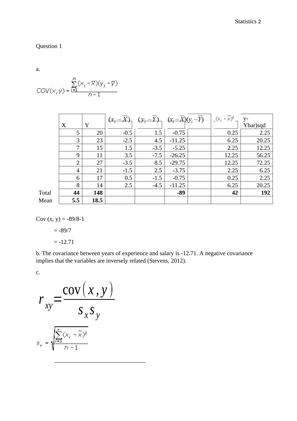
a.
X Y
y-
Ybar)sqd
5 20 -0.5 1.5 -0.75 0.25 2.25
3 23 -2.5 4.5 -11.25 6.25 20.25
7 15 1.5 -3.5 -5.25 2.25 12.25
9 11 3.5 -7.5 -26.25 12.25 56.25
2 27 -3.5 8.5 -29.75 12.25 72.25
4 21 -1.5 2.5 -3.75 2.25 6.25
6 17 0.5 -1.5 -0.75 0.25 2.25
8 14 2.5 -4.5 -11.25 6.25 20.25
Total 44 148 -89 42 192
Mean 5.5 18.5
Cov (x, y) = -89/8-1
= -89/7
= -12.71
b. The covariance between years of experience and salary is -12.71. A negative covariance
implies that the variables are inversely related (Stevens, 2012).
c.
r xy=cov ( x , y )
s x s y

Statistics 3
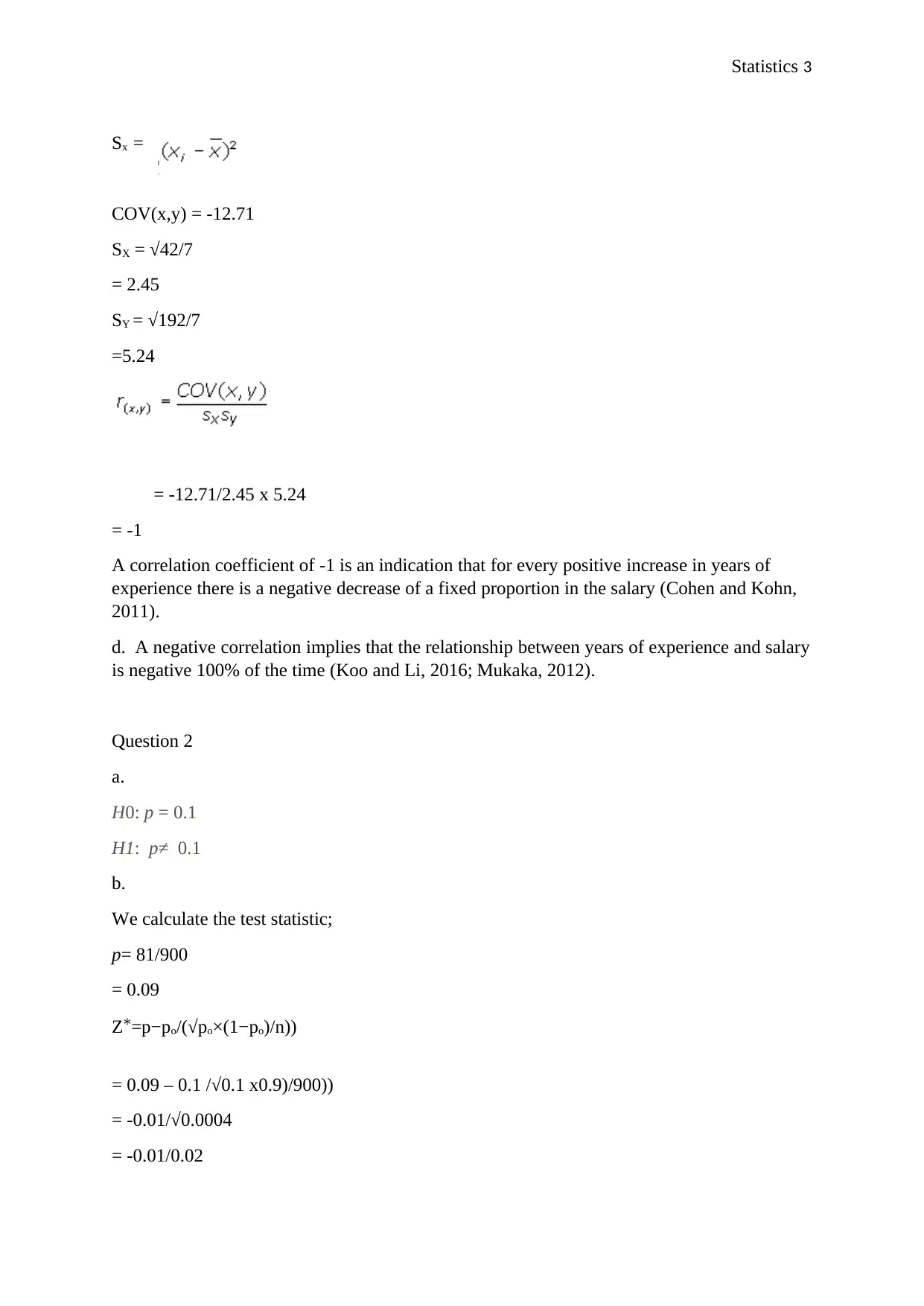
Sx =
COV(x,y) = -12.71
SX = √42/7
= 2.45
SY = √192/7
=5.24
= -12.71/2.45 x 5.24
= -1
A correlation coefficient of -1 is an indication that for every positive increase in years of
experience there is a negative decrease of a fixed proportion in the salary (Cohen and Kohn,
2011).
d. A negative correlation implies that the relationship between years of experience and salary
is negative 100% of the time (Koo and Li, 2016; Mukaka, 2012).
Question 2
a.
H0: p = 0.1
H1: p≠ 0.1
b.
We calculate the test statistic;
p= 81/900
= 0.09
Z∗=p−po/(√po×(1−po)/n))
= 0.09 – 0.1 /√0.1 x0.9)/900))
= -0.01/√0.0004
= -0.01/0.02

Statistics 4
Z∗=- 0.5
We next ascertain the region of rejection for the level of significance and also the p-value for
the test statistic;
From the Z-table and alpha value of 0.025;
Z = -2.81
Since the test statistic Z∗ of – 0.5 falls outside the area of rejection (more than -2.81), the null
hypothesis is accepted
With the p-value close to zero and being more than alpha of 0.05, we accept the null
hypothesis. There is statistical evidence at 5% significance level to conclude that 10% of the
users of a certain sinus drug experience drowsiness.
c.
CI = [X¯ − tα/2 σ √ n , X¯ + tα/2 σ √ n ]
SEX¯ = s √ n
=81/√900
= 2.7
= tα/2,n−1 = 2.045
CI = 81 – 2.045 X2.7, 81 + 2.045 X 2.7
= 75.48, 86.52)
= (75, 87)
d. If the confidence interval has the value claimed by the null hypothesis, then the findings
are close to the claimed value, hence null hypothesis is not rejected (Javanmard and
Montanari, 2014; Greenland et al., 2016).
On the other hand if the interval doesn’t have the claimed value by the HO, then the findings
vary significantly from the claimed value, thus null hypothesis is rejected (Murphy, Myors,
and Wolach, 2014; Siegmund, 2013).
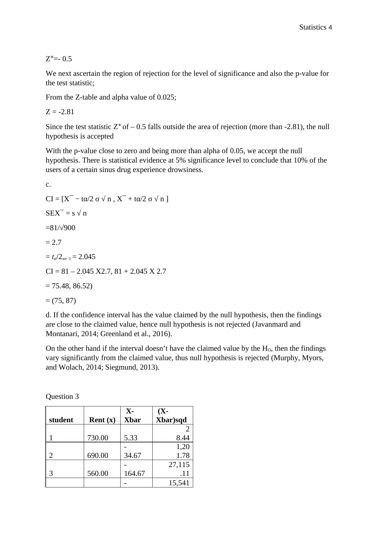
Question 3
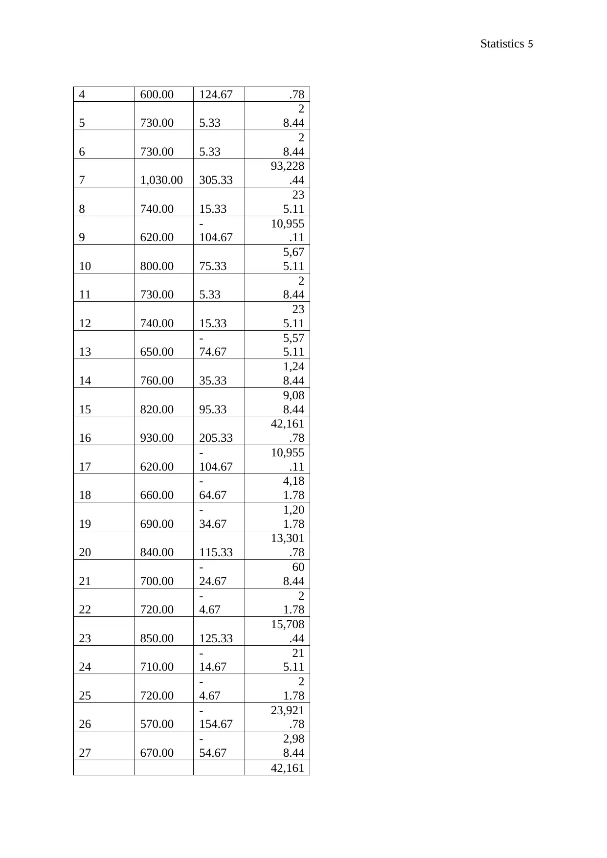
student Rent (x)
X-
Xbar
(X-
Xbar)sqd
1 730.00 5.33
2
8.44
2 690.00
-
34.67
1,20
1.78
3 560.00
-
164.67
27,115
.11
- 15,541

Statistics 5
4 600.00 124.67 .78
5 730.00 5.33
2
8.44
6 730.00 5.33
2
8.44
7 1,030.00 305.33
93,228
.44
8 740.00 15.33
23
5.11
9 620.00
-
104.67
10,955
.11
10 800.00 75.33
5,67
5.11
11 730.00 5.33
2
8.44
12 740.00 15.33
23
5.11
13 650.00
-
74.67
5,57
5.11
14 760.00 35.33
1,24
8.44
15 820.00 95.33
9,08
8.44
16 930.00 205.33
42,161
.78
17 620.00
-
104.67
10,955
.11
18 660.00
-
64.67
4,18
1.78
19 690.00
-
34.67
1,20
1.78
20 840.00 115.33
13,301
.78
21 700.00
-
24.67
60
8.44
22 720.00
-
4.67
2
1.78
23 850.00 125.33
15,708
.44
24 710.00
-
14.67
21
5.11
25 720.00
-
4.67
2
1.78
26 570.00
-
154.67
23,921
.78
27 670.00
-
54.67
2,98
8.44
42,161

Statistics 6
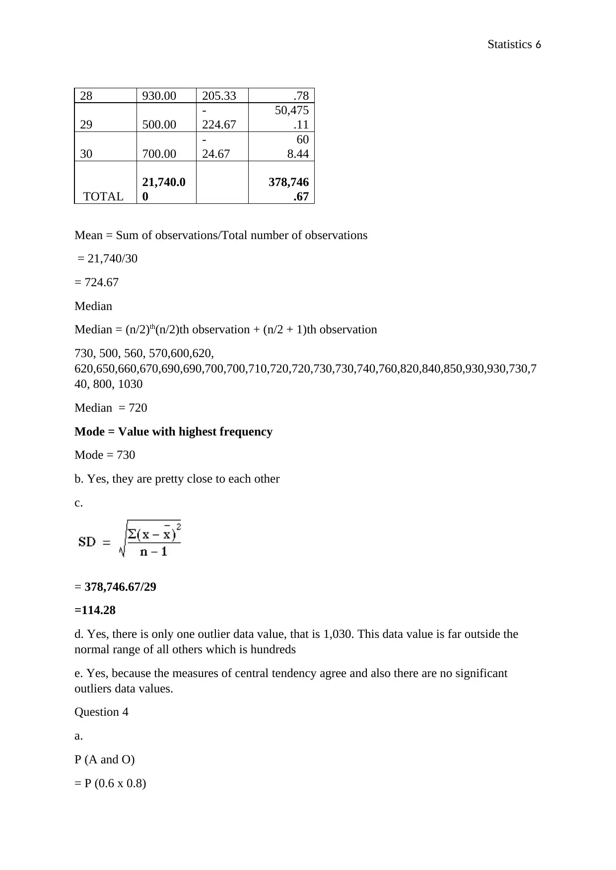
28 930.00 205.33 .78
29 500.00
-
224.67
50,475
.11
30 700.00
-
24.67
60
8.44
TOTAL
21,740.0
0
378,746
.67
Mean = Sum of observations/Total number of observations
= 21,740/30
= 724.67
Median
Median = (n/2)th(n/2)th observation + (n/2 + 1)th observation
730, 500, 560, 570,600,620,
620,650,660,670,690,690,700,700,710,720,720,730,730,740,760,820,840,850,930,930,730,7
40, 800, 1030
Median = 720
Mode = Value with highest frequency
Mode = 730
b. Yes, they are pretty close to each other
c.
= 378,746.67/29
=114.28
d. Yes, there is only one outlier data value, that is 1,030. This data value is far outside the
normal range of all others which is hundreds
e. Yes, because the measures of central tendency agree and also there are no significant
outliers data values.
Question 4
a.
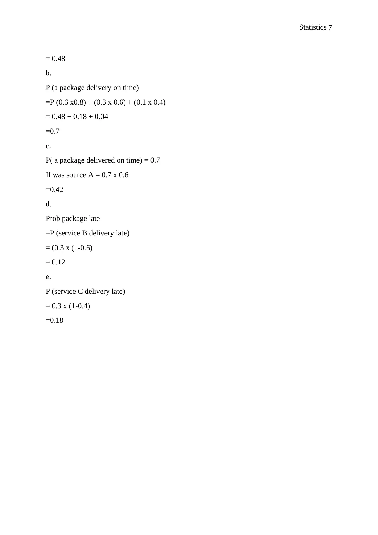
P (A and O)
= P (0.6 x 0.8)

Statistics 7
= 0.48
b.
P (a package delivery on time)
=P (0.6 x0.8) + (0.3 x 0.6) + (0.1 x 0.4)
= 0.48 + 0.18 + 0.04
=0.7
c.
P( a package delivered on time) = 0.7
If was source A = 0.7 x 0.6
=0.42
d.
Prob package late
=P (service B delivery late)
= (0.3 x (1-0.6)
= 0.12
e.
P (service C delivery late)
= 0.3 x (1-0.4)
=0.18

Statistics 8
References
Cohen, M.R. and Kohn, A., 2011. Measuring and interpreting neuronal correlations. Nature
neuroscience, 14(7), p.811.
Greenland, S., Senn, S.J., Rothman, K.J., Carlin, J.B., Poole, C., Goodman, S.N. and Altman,
D.G., 2016. Statistical tests, P values, confidence intervals, and power: a guide to
misinterpretations. European journal of epidemiology, 31(4), pp.337-350.
Javanmard, A. and Montanari, A., 2014. Confidence intervals and hypothesis testing for high-
dimensional regression. The Journal of Machine Learning Research, 15(1), pp.2869-2909.
Koo, T.K. and Li, M.Y., 2016. A guideline of selecting and reporting intraclass correlation
coefficients for reliability research. Journal of chiropractic medicine, 15(2), pp.155-163.
Mukaka, M.M., 2012. A guide to appropriate use of correlation coefficient in medical
research. Malawi Medical Journal, 24(3), pp.69-71.
Murphy, K.R., Myors, B. and Wolach, A., 2014. Statistical power analysis: A simple and
general model for traditional and modern hypothesis tests. Routledge.
Siegmund, D., 2013. Sequential analysis: tests and confidence intervals. Springer Science &
Business Media.
Stevens, J.P., 2012. Analysis of covariance. In Applied Multivariate Statistics for the Social
Sciences, Fifth Edition (pp. 299-326). Routledge.

Statistics 9