Creep and Fatigue: Secondary Creep Rate and Tensile Tests

This document discusses the secondary creep rate obtained from creep tests on aluminum alloy and tensile tests at various temperatures. It also calculates the initial tightening stress in bolts and safe range stress for repeated cycles using Gerber and Goodman fatigue predictions. The Weibull model and inverse power law model that describe the life-stress relationship function are also discussed.

FACULTY OF TECHNOLOGY
COURSE WORK SPECIFICATION 2018/2019
ADVANCED SOLID MECHANICS
ENGT5258/ENGD5258
CREEP & FATIGUE
ASSIGNMENT
2018
Institutional Affiliation
Student Name

CREEP & FATIGUE
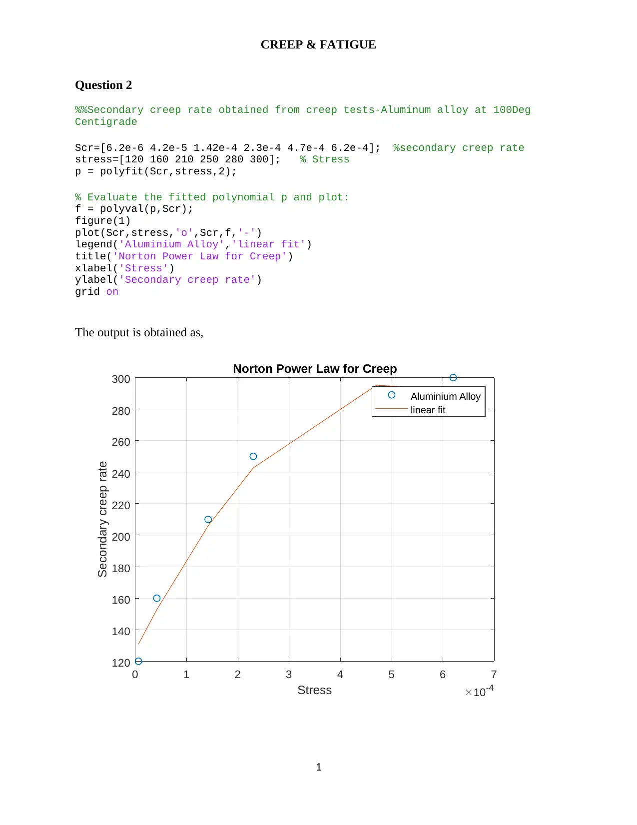
Question 2
%%Secondary creep rate obtained from creep tests-Aluminum alloy at 100Deg
Centigrade
Scr=[6.2e-6 4.2e-5 1.42e-4 2.3e-4 4.7e-4 6.2e-4]; %secondary creep rate
stress=[120 160 210 250 280 300]; % Stress
p = polyfit(Scr,stress,2);
% Evaluate the fitted polynomial p and plot:
f = polyval(p,Scr);
figure(1)
plot(Scr,stress,'o',Scr,f,'-')
legend('Aluminium Alloy','linear fit')
title('Norton Power Law for Creep')
xlabel('Stress')
ylabel('Secondary creep rate')
grid on
The output is obtained as,
0 1 2 3 4 5 6 7
Stress 10-4
120
140
160
180
200
220
240
260
280
300
Secondary creep rate
Norton Power Law for Creep
Aluminium Alloy
linear fit
1

CREEP & FATIGUE
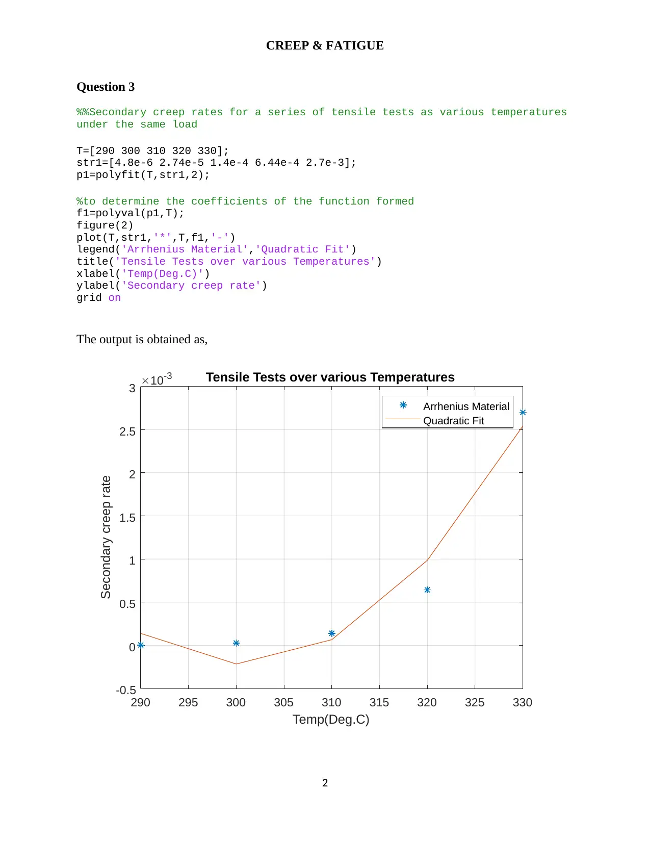
Question 3
%%Secondary creep rates for a series of tensile tests as various temperatures
under the same load
T=[290 300 310 320 330];
str1=[4.8e-6 2.74e-5 1.4e-4 6.44e-4 2.7e-3];
p1=polyfit(T,str1,2);
%to determine the coefficients of the function formed
f1=polyval(p1,T);
figure(2)
plot(T,str1,'*',T,f1,'-')
legend('Arrhenius Material','Quadratic Fit')
title('Tensile Tests over various Temperatures')
xlabel('Temp(Deg.C)')
ylabel('Secondary creep rate')
grid on
The output is obtained as,
290 295 300 305 310 315 320 325 330
Temp(Deg.C)
-0.5
0
0.5
1
1.5
2
2.5
3
Secondary creep rate
10-3 Tensile Tests over various Temperatures
Arrhenius Material
Quadratic Fit
2

CREEP & FATIGUE
Question 4
In a cylindrical vessel,
Pressure 1.5MPa
Cover plate diameter 450mm
30 bolts of 20mm diameter (equally spaced around the rim)
E=210GPa
Secondary creep rate= 32.2e-17
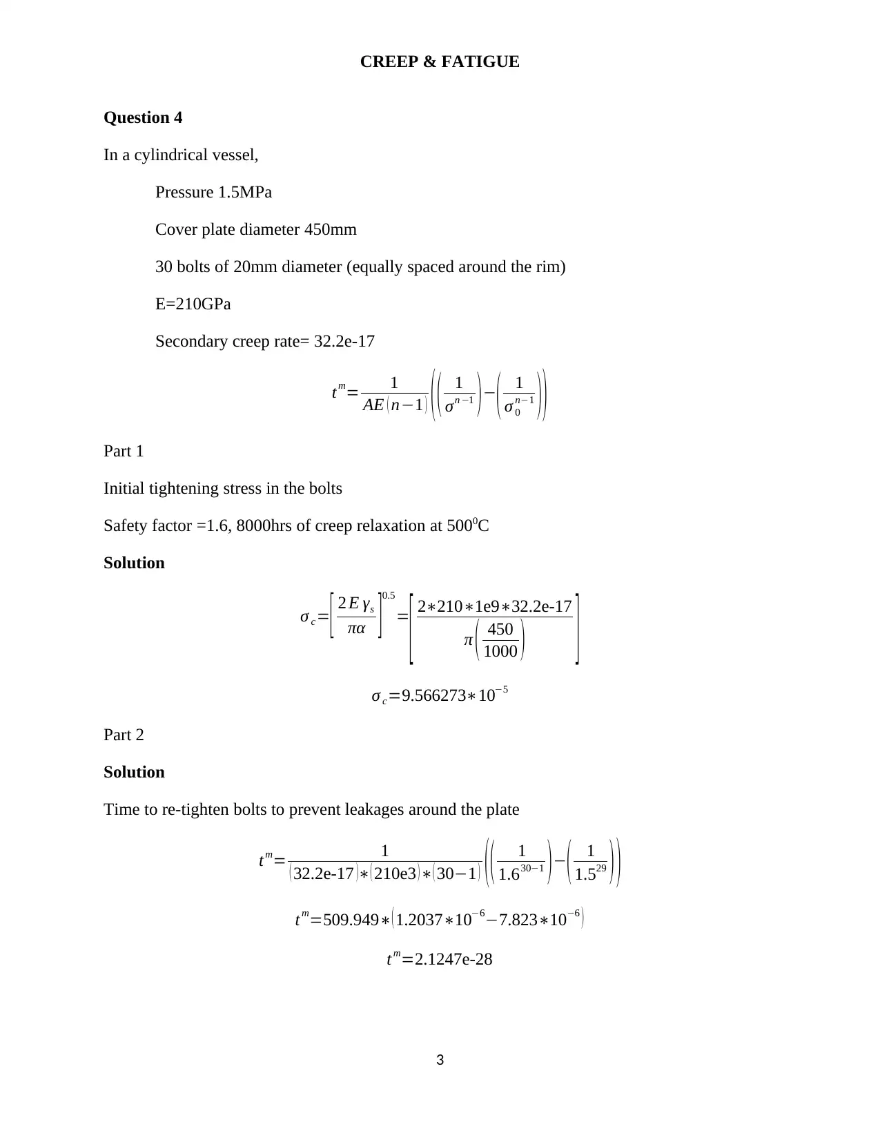
tm= 1
AE ( n−1 ) ( ( 1
σn −1 ) −
( 1
σ 0
n−1 ))
Part 1
Initial tightening stress in the bolts
Safety factor =1.6, 8000hrs of creep relaxation at 5000C
Solution
σ c=[ 2 E γs
πα ]
0.5
=
[ 2∗210∗1e9∗32.2e-17
π ( 450
1000 ) ]
σ c=9.566273∗10−5
Part 2
Solution
Time to re-tighten bolts to prevent leakages around the plate
tm= 1
( 32.2e-17 )∗( 210e3 )∗( 30−1 ) (( 1
1.630−1 )−
( 1
1.529 ) )
tm=509.949∗( 1.2037∗10−6−7.823∗10−6 )
tm=2.1247e-28
3

CREEP & FATIGUE
Question 6
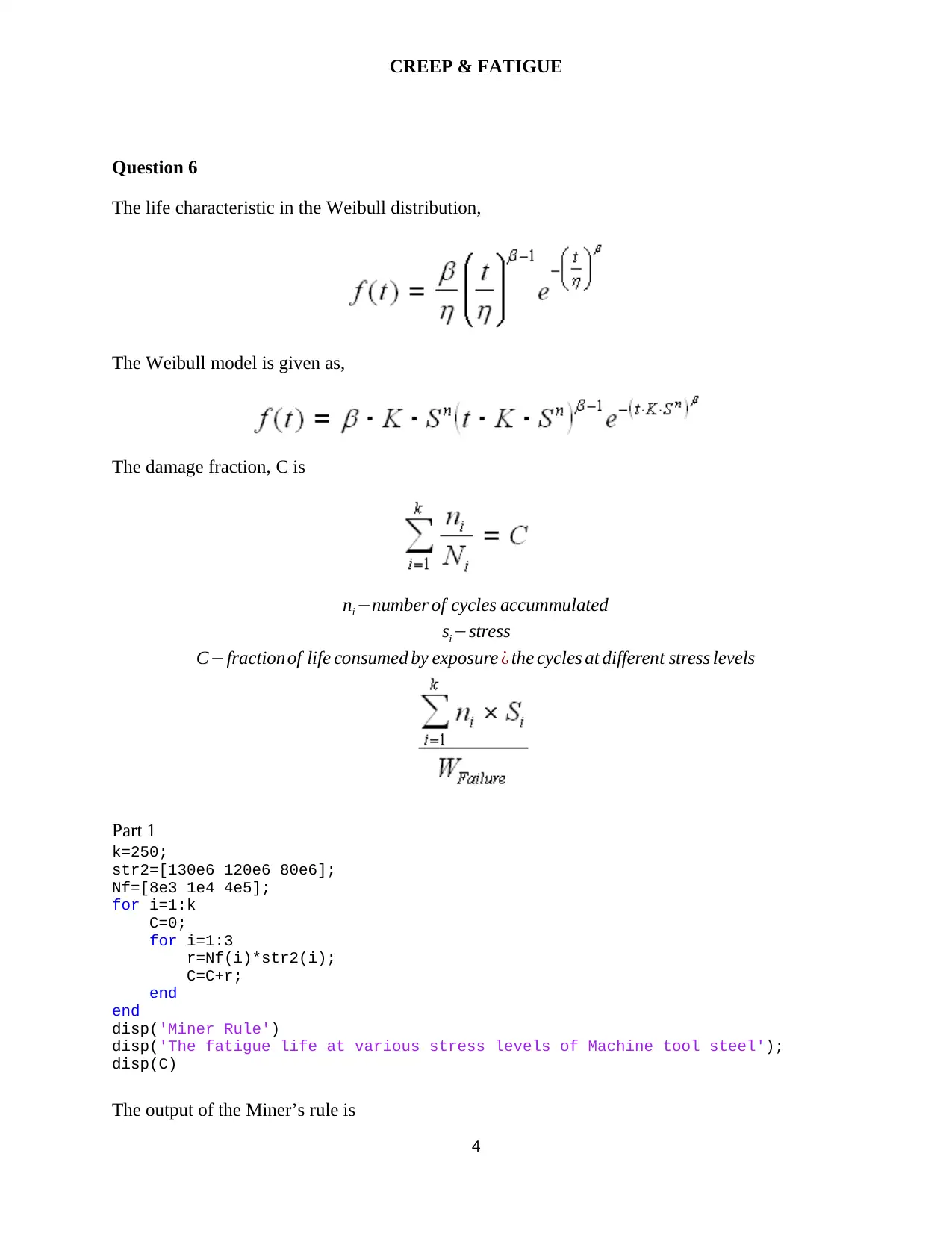
The life characteristic in the Weibull distribution,
The Weibull model is given as,
The damage fraction, C is
ni −number of cycles accummulated
si−stress
C−fractionof life consumed by exposure ¿ the cycles at different stress levels
Part 1
k=250;
str2=[130e6 120e6 80e6];
Nf=[8e3 1e4 4e5];
for i=1:k
C=0;
for i=1:3
r=Nf(i)*str2(i);
C=C+r;
end
end
disp('Miner Rule')
disp('The fatigue life at various stress levels of Machine tool steel');
disp(C)
The output of the Miner’s rule is
4

CREEP & FATIGUE
¿ ( ( 130∗8 ) + ( 120∗10 )+ ( 80∗400 ) )
250
¿ 136.96
Part 2
Using the non-linear approach where damage curves.
To determine the inverse power law model that describes the life-stress relationship function as,
L ( s )= 1
K Sn
The equivalent stress on the damage curves is given as,
Seq=B1 ( P Dext
2t )+ B2 ( DExt
2 I ) M
Question 7
Reverse stress fatigue limit for low-carbon steel
± 270 MPa
UTS=670 MPa
yield stress=260 MP a
Part 1
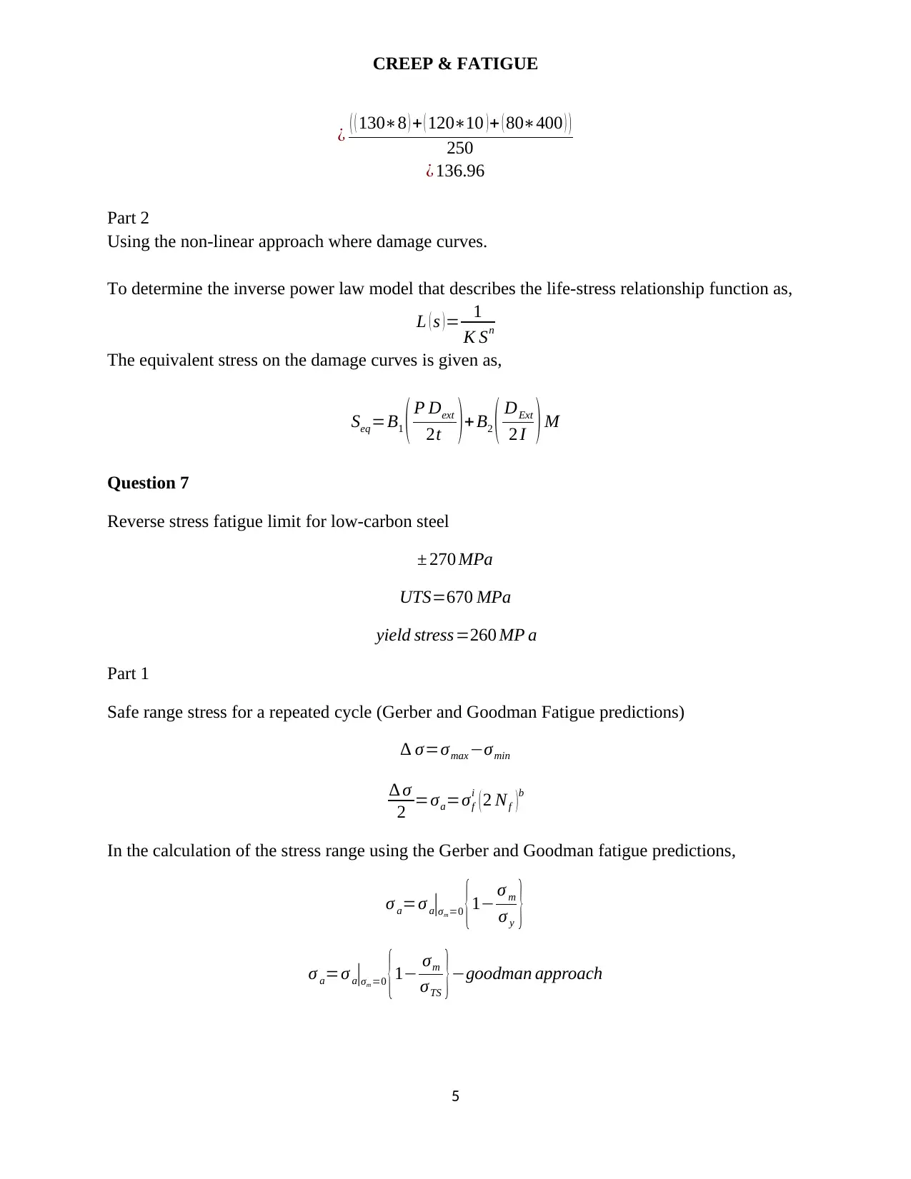
Safe range stress for a repeated cycle (Gerber and Goodman Fatigue predictions)
∆ σ=σmax−σmin
∆ σ
2 =σa=σf
i
( 2 Nf )b
In the calculation of the stress range using the Gerber and Goodman fatigue predictions,
σ a=σ a|σm =0 {1− σ m
σ y }
σ a=σ a|σm =0 {1− σm
σTS }−goodman approach
5

CREEP & FATIGUE
σ a=σ a|σm =0 {1− ( σm
σTS )2
}−Gerber approach
Part 2
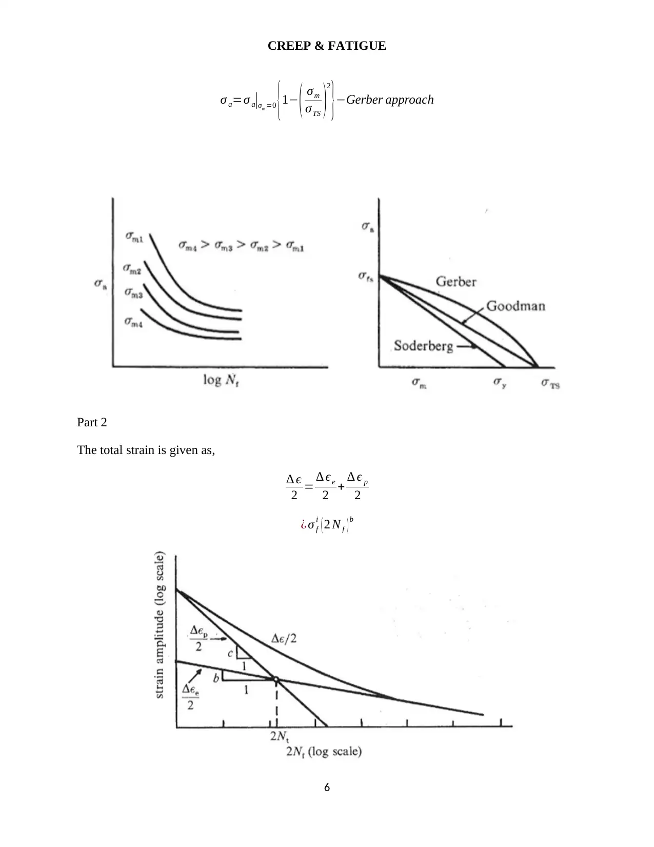
The total strain is given as,
∆ ϵ
2 = ∆ ϵe
2 + ∆ ϵ p
2
¿ σ f
i
( 2 N f ) b
6