Naive Bayes Classification of Ionosphere Dataset

The assignment content provided involves the use of naive Bayes classifiers to perform calculations and predictions. The Bayes theorem is applied to obtain conditional probabilities from a sample dataset. Additionally, there is a Matlab function `myNeuralNetworkFunction` that simulates a neural network using inbuilt functions such as `negdist_apply` and `compet_apply`. Furthermore, the assignment includes the solution of a clustering problem using Self-Organizing Map (SOM) algorithm.

DEPARTMENT OF COMPUTER SCIENCE AND INFORMATION TECHNOLOGY
LA TOBRE UNIVERSITY
CSE5DMI DATA MINING
ASSIGNMENT TWO
STUDENT NAME
STUDENT REGISTRATION NUMBER
DATE OF SUBMISSION

DATA MINING
Question 1
(a) Create trained and test data in a Matlab function
70% of the dataset used for training
30% of the dataset used for testing
There are four matrices such that there are two class labels datasets and two attribute
value data sets.
Task 1: Data preparation
The wine quality dataset is loaded into the MATLAB workspace,
[wineQtrain, wineQattr]=wine_dataset;
The attribute values are split into training and test datasets
Train_wineQ=wineQtrain(:,[1:500 601:1400 1601:1900]);
Test_wineQ=wineQtrain(:,[501:600 1401:1600 1901:2000]);
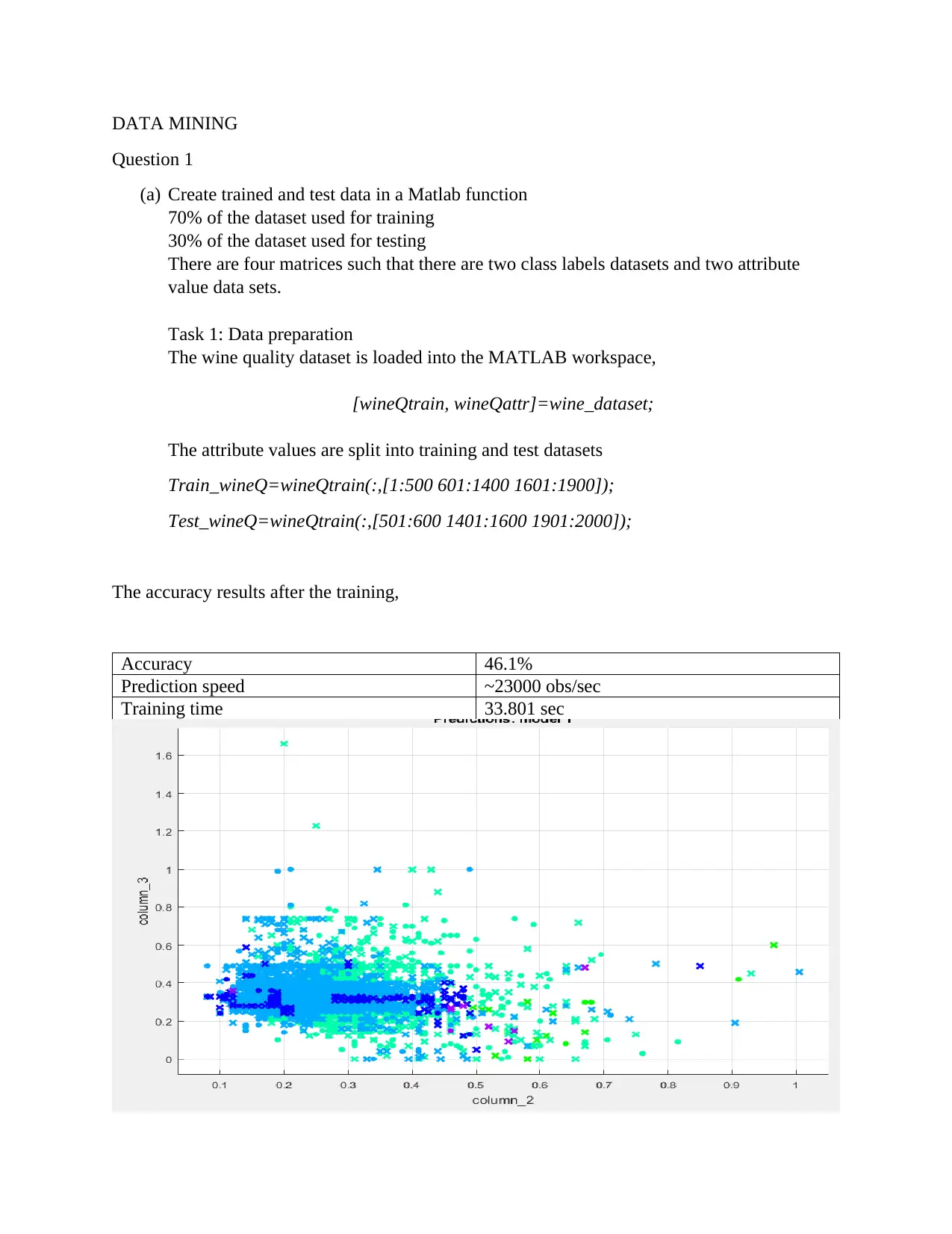
The accuracy results after the training,
Accuracy 46.1%
Prediction speed ~23000 obs/sec
Training time 33.801 sec

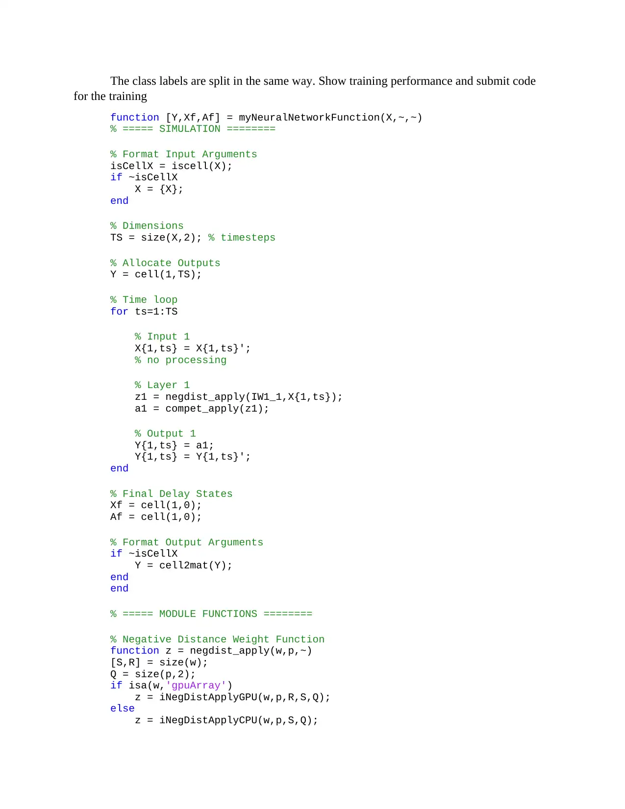
The class labels are split in the same way. Show training performance and submit code
for the training
function [Y,Xf,Af] = myNeuralNetworkFunction(X,~,~)
% ===== SIMULATION ========
% Format Input Arguments
isCellX = iscell(X);
if ~isCellX
X = {X};
end
% Dimensions
TS = size(X,2); % timesteps
% Allocate Outputs
Y = cell(1,TS);
% Time loop
for ts=1:TS
% Input 1
X{1,ts} = X{1,ts}';
% no processing
% Layer 1
z1 = negdist_apply(IW1_1,X{1,ts});
a1 = compet_apply(z1);
% Output 1
Y{1,ts} = a1;
Y{1,ts} = Y{1,ts}';
end
% Final Delay States
Xf = cell(1,0);
Af = cell(1,0);
% Format Output Arguments
if ~isCellX
Y = cell2mat(Y);
end
end
% ===== MODULE FUNCTIONS ========
% Negative Distance Weight Function
function z = negdist_apply(w,p,~)
[S,R] = size(w);
Q = size(p,2);
if isa(w,'gpuArray')
z = iNegDistApplyGPU(w,p,R,S,Q);
else
z = iNegDistApplyCPU(w,p,S,Q);

end
end
function z = iNegDistApplyCPU(w,p,S,Q)
z = zeros(S,Q);
if (Q<S)
pt = p';
for q=1:Q
z(:,q) = sum(bsxfun(@minus,w,pt(q,:)).^2,2);
end
else
wt = w';
for i=1:S
z(i,:) = sum(bsxfun(@minus,wt(:,i),p).^2,1);
end
end
z = -sqrt(z);
end
function z = iNegDistApplyGPU(w,p,R,S,Q)
p = reshape(p,1,R,Q);
sd = arrayfun(@iNegDistApplyGPUHelper,w,p);
z = -sqrt(reshape(sum(sd,2),S,Q));
end
function sd = iNegDistApplyGPUHelper(w,p)
sd = (w-p) .^ 2;
end
% Competitive Transfer Function
function a = compet_apply(n,~)
if isempty(n)
a = n;
else
[S,Q] = size(n);
nanInd = any(isnan(n),1);
a = zeros(S,Q,'like',n);
[~,maxRows] = max(n,[],1);
onesInd = maxRows + S*(0:(Q-1));
a(onesInd) = 1;
a(:,nanInd) = NaN;
end
end
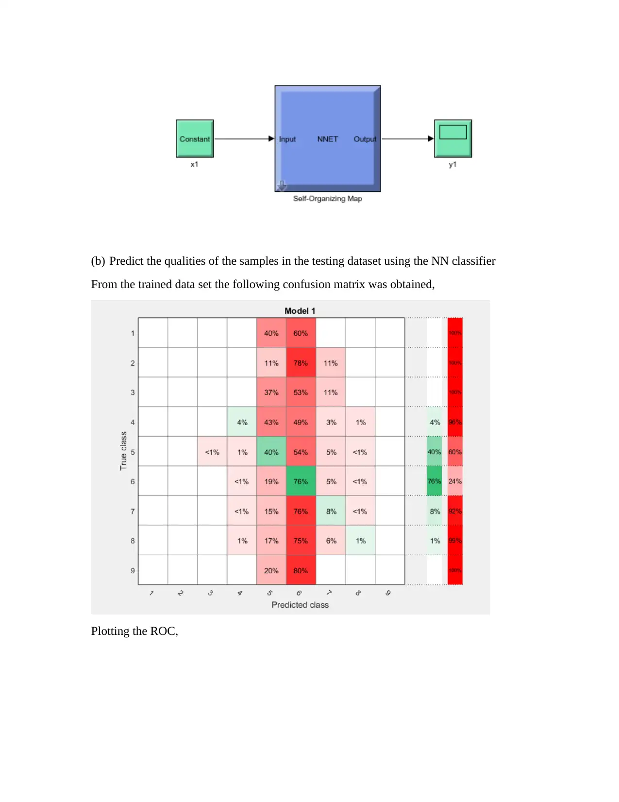
Deploying the solution, one can obtain the Simulink neural network diagram as,

(b) Predict the qualities of the samples in the testing dataset using the NN classifier
From the trained data set the following confusion matrix was obtained,
Plotting the ROC,

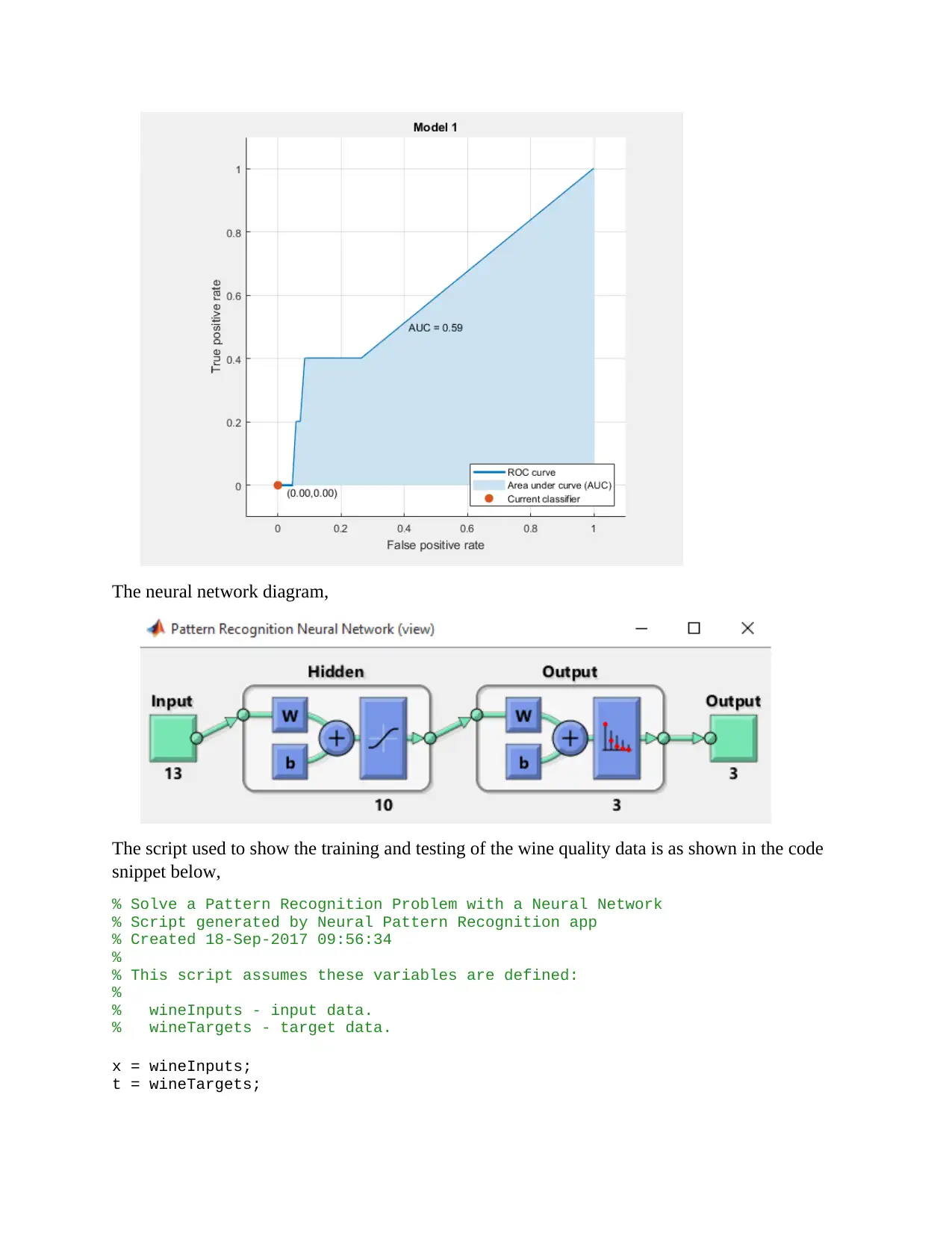
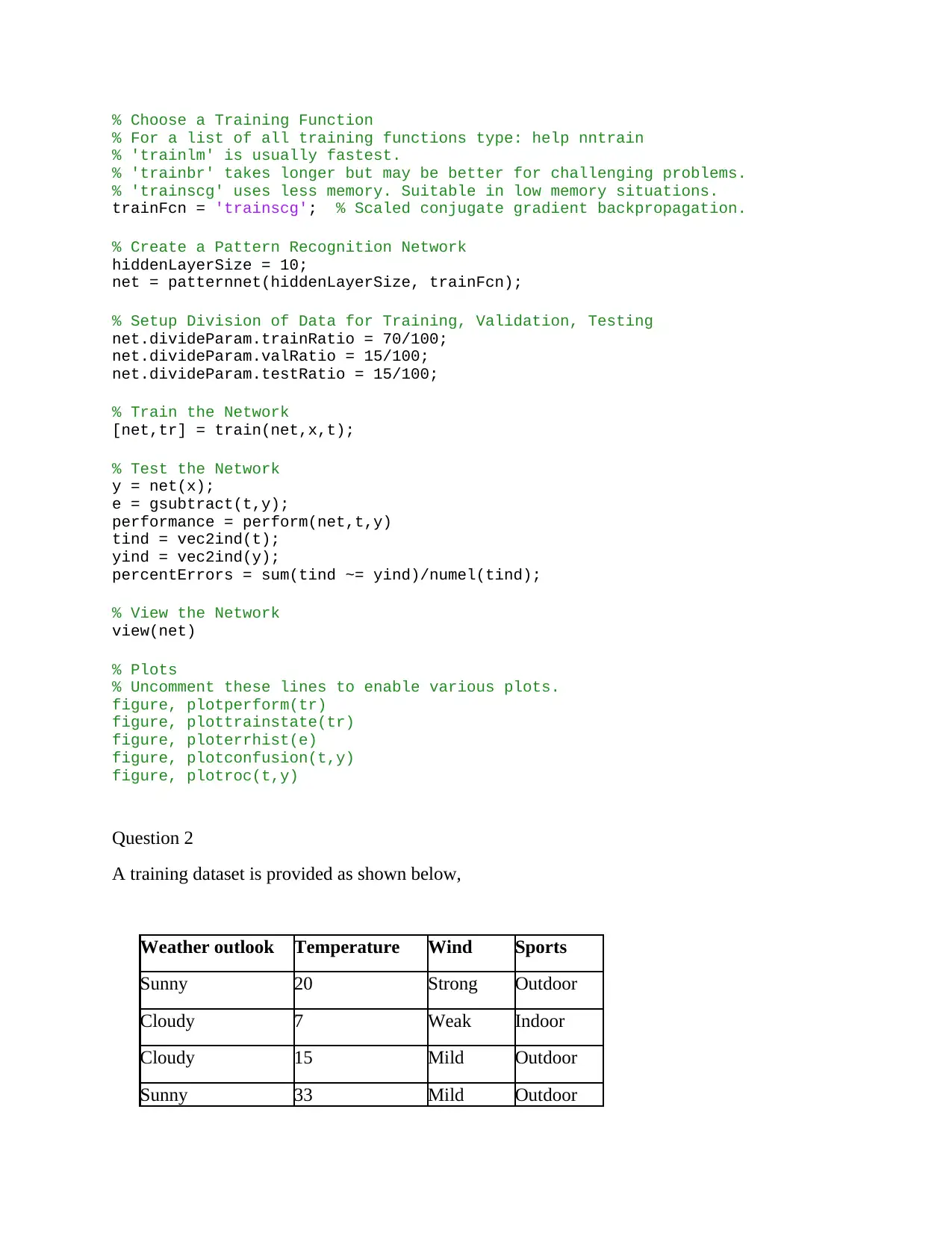
The neural network diagram,
The script used to show the training and testing of the wine quality data is as shown in the code
snippet below,
% Solve a Pattern Recognition Problem with a Neural Network
% Script generated by Neural Pattern Recognition app
% Created 18-Sep-2017 09:56:34
%
% This script assumes these variables are defined:
%
% wineInputs - input data.
% wineTargets - target data.
x = wineInputs;
t = wineTargets;

% Choose a Training Function
% For a list of all training functions type: help nntrain
% 'trainlm' is usually fastest.
% 'trainbr' takes longer but may be better for challenging problems.
% 'trainscg' uses less memory. Suitable in low memory situations.
trainFcn = 'trainscg'; % Scaled conjugate gradient backpropagation.
% Create a Pattern Recognition Network
hiddenLayerSize = 10;
net = patternnet(hiddenLayerSize, trainFcn);
% Setup Division of Data for Training, Validation, Testing
net.divideParam.trainRatio = 70/100;
net.divideParam.valRatio = 15/100;
net.divideParam.testRatio = 15/100;
% Train the Network
[net,tr] = train(net,x,t);
% Test the Network
y = net(x);
e = gsubtract(t,y);
performance = perform(net,t,y)
tind = vec2ind(t);
yind = vec2ind(y);
percentErrors = sum(tind ~= yind)/numel(tind);
% View the Network
view(net)
% Plots
% Uncomment these lines to enable various plots.
figure, plotperform(tr)
figure, plottrainstate(tr)
figure, ploterrhist(e)
figure, plotconfusion(t,y)
figure, plotroc(t,y)
Question 2
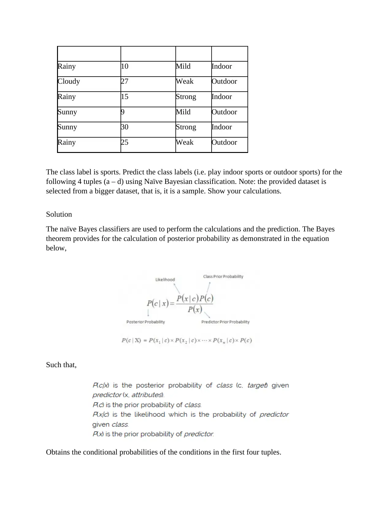
A training dataset is provided as shown below,
Weather outlook Temperature Wind Sports
Sunny 20 Strong Outdoor
Cloudy 7 Weak Indoor
Cloudy 15 Mild Outdoor
Sunny 33 Mild Outdoor

Rainy 10 Mild Indoor
Cloudy 27 Weak Outdoor
Rainy 15 Strong Indoor
Sunny 9 Mild Outdoor
Sunny 30 Strong Indoor
Rainy 25 Weak Outdoor
The class label is sports. Predict the class labels (i.e. play indoor sports or outdoor sports) for the
following 4 tuples (a – d) using Naïve Bayesian classification. Note: the provided dataset is
selected from a bigger dataset, that is, it is a sample. Show your calculations.
Solution
The naïve Bayes classifiers are used to perform the calculations and the prediction. The Bayes
theorem provides for the calculation of posterior probability as demonstrated in the equation
below,
Such that,
Obtains the conditional probabilities of the conditions in the first four tuples.

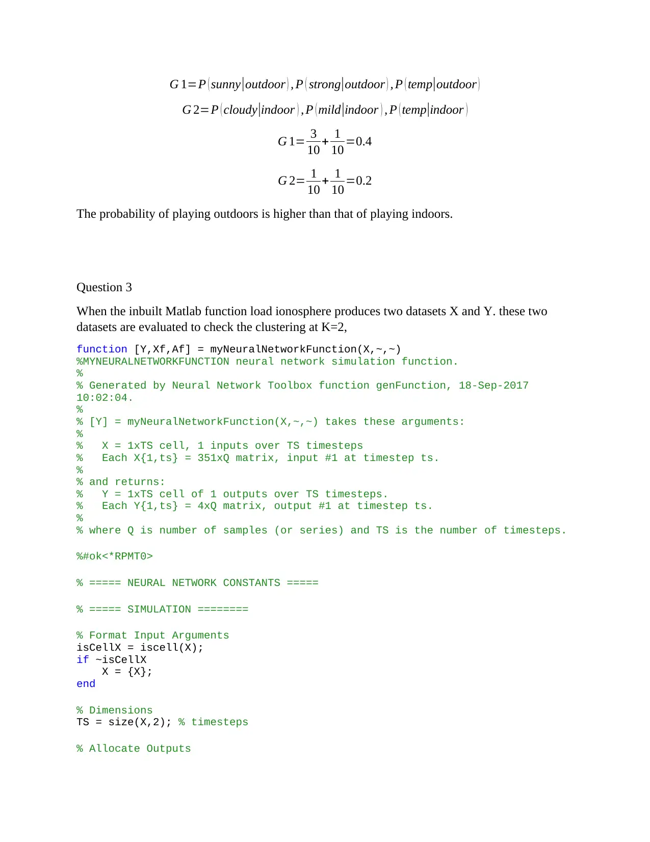
G 1=P ( sunny|outdoor ) , P ( strong|outdoor ) , P ( temp|outdoor )
G 2=P ( cloudy|indoor ) , P ( mild|indoor ) , P ( temp|indoor )
G 1= 3
10 + 1
10 =0.4
G 2= 1
10 + 1
10 =0.2
The probability of playing outdoors is higher than that of playing indoors.
Question 3
When the inbuilt Matlab function load ionosphere produces two datasets X and Y. these two
datasets are evaluated to check the clustering at K=2,
function [Y,Xf,Af] = myNeuralNetworkFunction(X,~,~)
%MYNEURALNETWORKFUNCTION neural network simulation function.
%
% Generated by Neural Network Toolbox function genFunction, 18-Sep-2017
10:02:04.
%
% [Y] = myNeuralNetworkFunction(X,~,~) takes these arguments:
%
% X = 1xTS cell, 1 inputs over TS timesteps
% Each X{1,ts} = 351xQ matrix, input #1 at timestep ts.
%
% and returns:
% Y = 1xTS cell of 1 outputs over TS timesteps.
% Each Y{1,ts} = 4xQ matrix, output #1 at timestep ts.
%
% where Q is number of samples (or series) and TS is the number of timesteps.
%#ok<*RPMT0>
% ===== NEURAL NETWORK CONSTANTS =====
% ===== SIMULATION ========
% Format Input Arguments
isCellX = iscell(X);
if ~isCellX
X = {X};
end
% Dimensions
TS = size(X,2); % timesteps
% Allocate Outputs

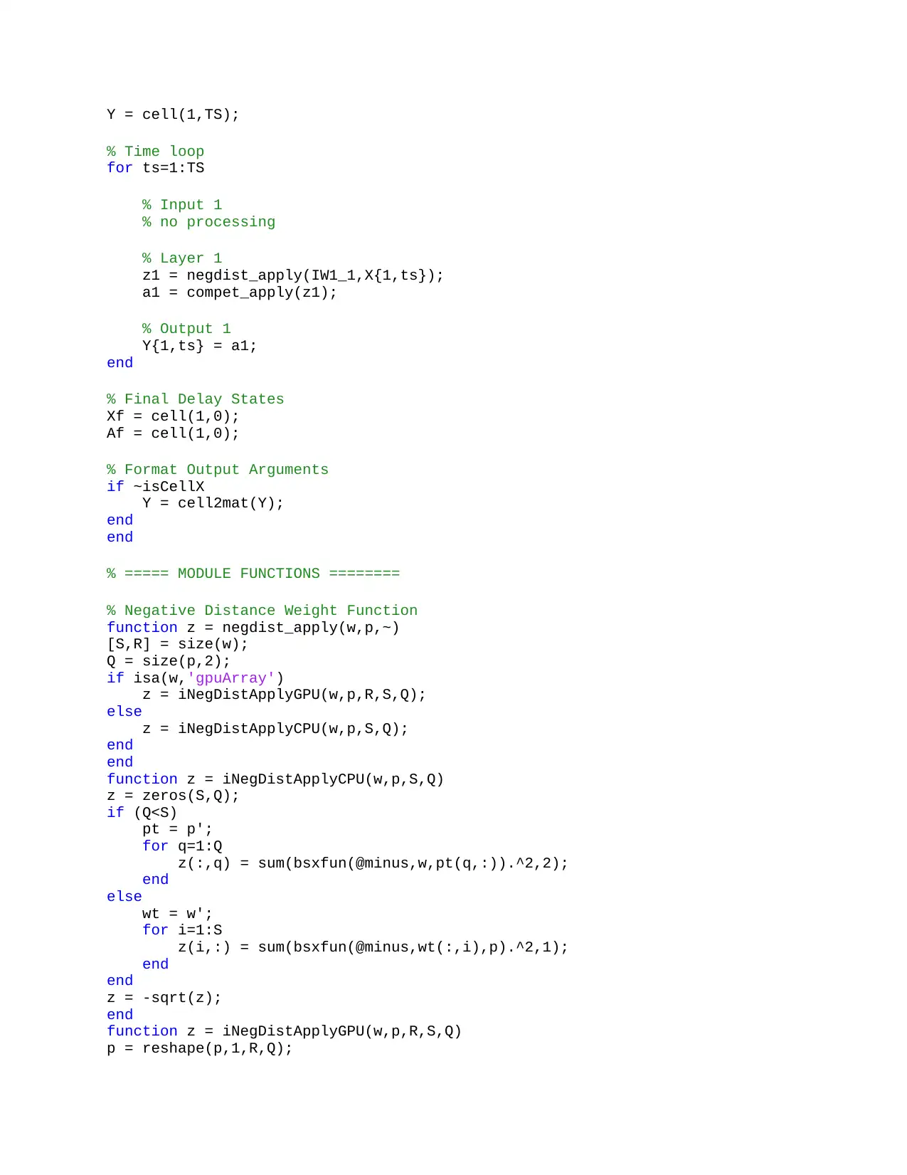
Y = cell(1,TS);
% Time loop
for ts=1:TS
% Input 1
% no processing
% Layer 1
z1 = negdist_apply(IW1_1,X{1,ts});
a1 = compet_apply(z1);
% Output 1
Y{1,ts} = a1;
end
% Final Delay States
Xf = cell(1,0);
Af = cell(1,0);
% Format Output Arguments
if ~isCellX
Y = cell2mat(Y);
end
end
% ===== MODULE FUNCTIONS ========
% Negative Distance Weight Function
function z = negdist_apply(w,p,~)
[S,R] = size(w);
Q = size(p,2);
if isa(w,'gpuArray')
z = iNegDistApplyGPU(w,p,R,S,Q);
else
z = iNegDistApplyCPU(w,p,S,Q);
end
end
function z = iNegDistApplyCPU(w,p,S,Q)
z = zeros(S,Q);
if (Q<S)
pt = p';
for q=1:Q
z(:,q) = sum(bsxfun(@minus,w,pt(q,:)).^2,2);
end
else
wt = w';
for i=1:S
z(i,:) = sum(bsxfun(@minus,wt(:,i),p).^2,1);
end
end
z = -sqrt(z);
end
function z = iNegDistApplyGPU(w,p,R,S,Q)
p = reshape(p,1,R,Q);

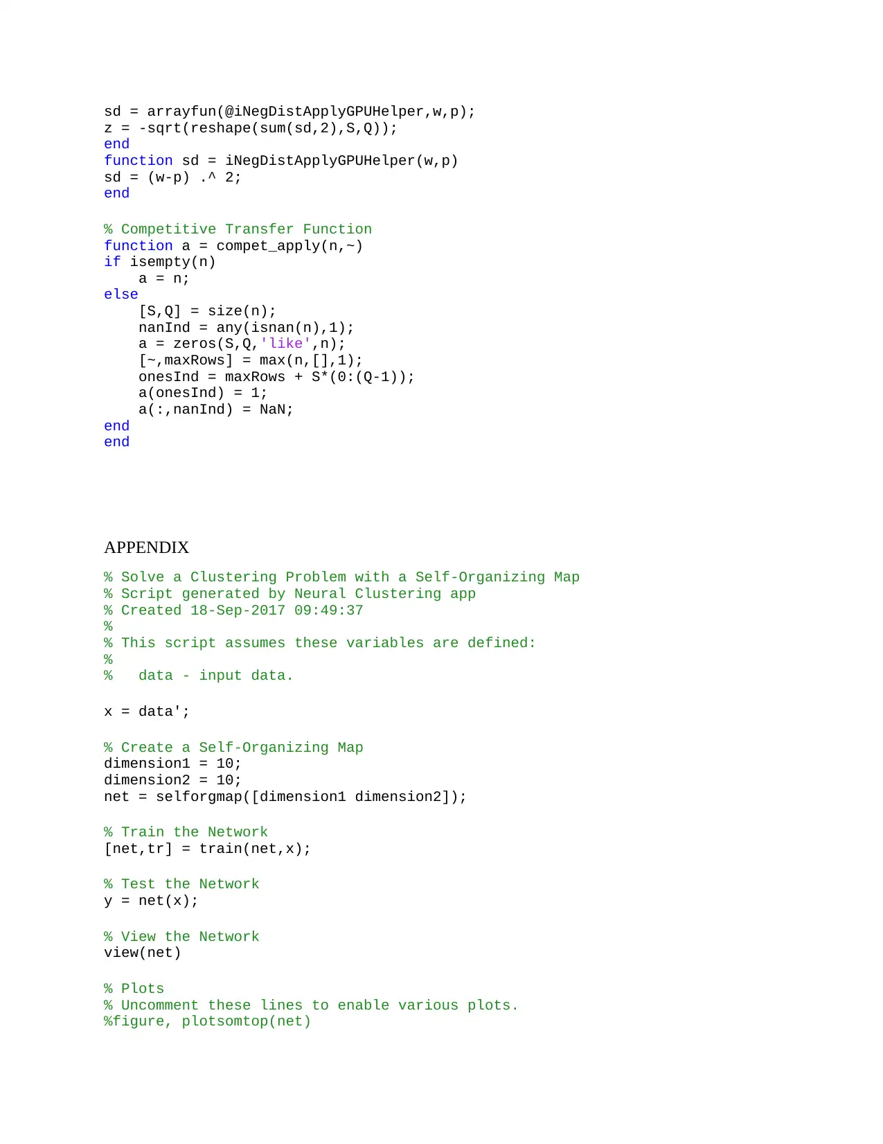
sd = arrayfun(@iNegDistApplyGPUHelper,w,p);
z = -sqrt(reshape(sum(sd,2),S,Q));
end
function sd = iNegDistApplyGPUHelper(w,p)
sd = (w-p) .^ 2;
end
% Competitive Transfer Function
function a = compet_apply(n,~)
if isempty(n)
a = n;
else
[S,Q] = size(n);
nanInd = any(isnan(n),1);
a = zeros(S,Q,'like',n);
[~,maxRows] = max(n,[],1);
onesInd = maxRows + S*(0:(Q-1));
a(onesInd) = 1;
a(:,nanInd) = NaN;
end
end
APPENDIX
% Solve a Clustering Problem with a Self-Organizing Map
% Script generated by Neural Clustering app
% Created 18-Sep-2017 09:49:37
%
% This script assumes these variables are defined:
%
% data - input data.
x = data';
% Create a Self-Organizing Map
dimension1 = 10;
dimension2 = 10;
net = selforgmap([dimension1 dimension2]);
% Train the Network
[net,tr] = train(net,x);
% Test the Network
y = net(x);
% View the Network
view(net)
% Plots
% Uncomment these lines to enable various plots.
%figure, plotsomtop(net)

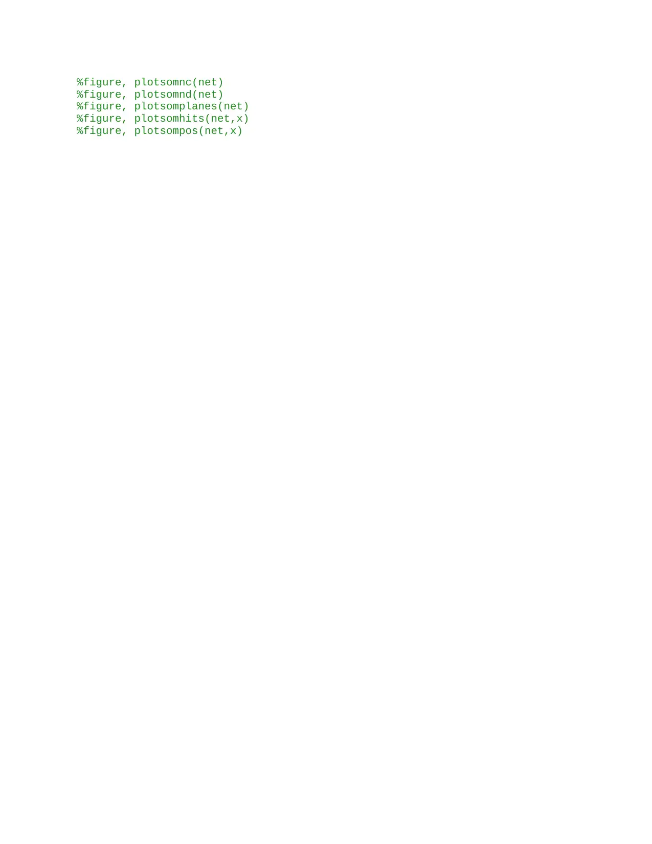
%figure, plotsomnc(net)
%figure, plotsomnd(net)
%figure, plotsomplanes(net)
%figure, plotsomhits(net,x)
%figure, plotsompos(net,x)