Data Analysis Techniques - Victoria

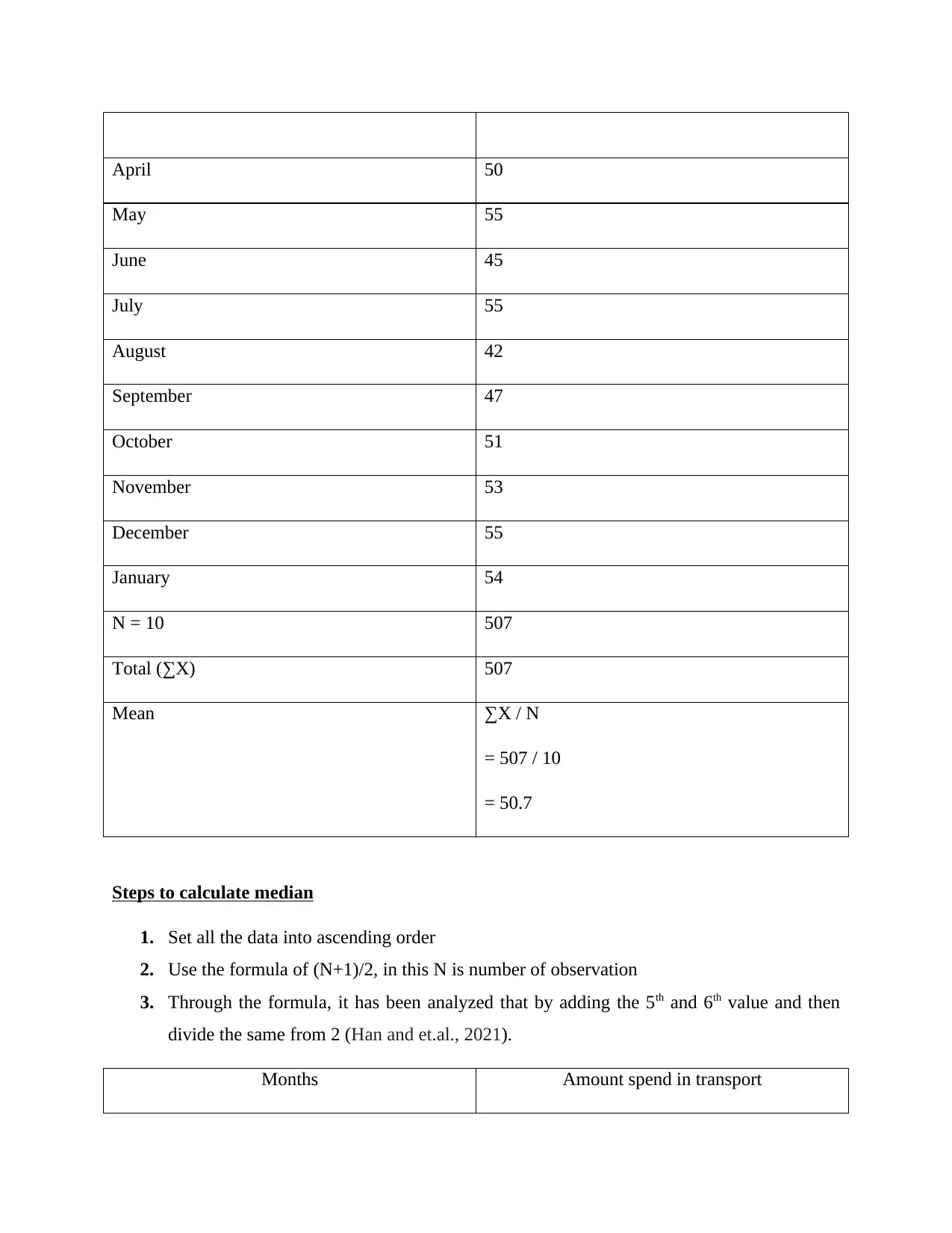
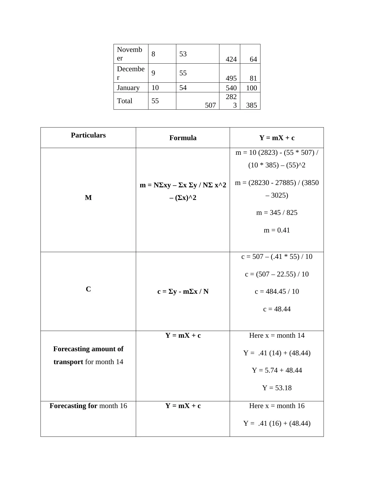
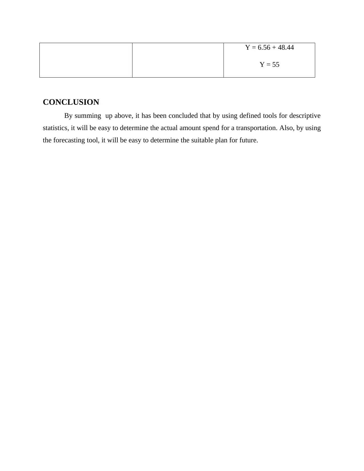
This study explores data analysis techniques and descriptive statistics for transportation spending. It presents the dataset in tabular and graphical form, calculates mean, median, mode, range, and standard deviation, and uses forecasting models to predict future spending. The study concludes that these tools are useful for determining actual spending and planning for the future.

Data analysis techniques - Victoria

TABLE OF CONTENTS
INTRODUCTION...........................................................................................................................2
Presenting the gathered dataset in a tabular format.....................................................................2
Present the data in graphical form...............................................................................................2
Describing the steps of descriptive statistics...............................................................................3
Calculating y = mx + c through forecasting model.....................................................................7
CONCLUSION................................................................................................................................9
REFERENCES..............................................................................................................................10

INTRODUCTION
Data analysis is all about to extract the useful information from the dataset in order to
determine the exact results. The present study is based upon the money spend upon
transportation from last ten months. The study will provide the deeper insight about the way in
which mean, mode, median used regarding amount spend upon transport.
Presenting the gathered dataset in a tabular format
Month Amount spend on transportation (£)
April 50
May 55
June 45
July 55
August 42
September 47
October 51
November 53
December 55
January 54
Present the data in graphical form
Bar graph:

April
May
June
July
August
September
October
November
December
January
0 10 20 30 40 50 60
50
55
45
55
42
47
51
53
55
54
Amount spend on transportation (Y)
Amount spend on
transportation (Y)
Line graph
April
May
June
July
August
September
October
November
December
January
0
10
20
30
40
50
60
50
55
45
55
42
47 51 53 55 54
Amount spend on transportation (Y)
Amount spend on
transportation (Y)
Describing the steps of descriptive statistics
Steps to calculate mean
1. Sum all the amount mentioned pertaining to amount spend upon transport
2. Evaluate the number of observation
3. Apply formula: Sum of amount spend upon transport / number of months (Thoen and
et.al., 2020)
Month Amount spend on transportation (£)

April 50
May 55
June 45
July 55
August 42
September 47
October 51
November 53
December 55
January 54
N = 10 507
Total (∑X) 507
Mean ∑X / N
= 507 / 10
= 50.7
Steps to calculate median
1. Set all the data into ascending order
2. Use the formula of (N+1)/2, in this N is number of observation
3. Through the formula, it has been analyzed that by adding the 5th and 6th value and then
divide the same from 2 (Han and et.al., 2021).
Months Amount spend in transport

August 42
June 45
September 47
April 50
October 51
November 53
January 54
December 55
July 55
May 55
Median = (N+1)/2 5.5
Median value (Value of 5th item + value of 6th item) / 2
= (51 + 53) / 2
= 52
Steps to calculate mode
In statistics, repetitive number is recognized as a mode. So 55 is repeat higher times and
that is why, it is consider as a mode.
Range
1. Identify the highest value and lowest value
2. Range is define as subtract the lowest value from highest
Highest value = 55
Lowest value = 42
Range = 55 – 42

= 13
Standard deviation
1. Determine the value of X^2 and then sum all
2. Perform sum of X^2 by number of observation (Gareiou and Zervas, 2018)
3. square of (∑x / n) is calculated
4. Subtract the outcome of 3 from 4
Month
Amount
spend on
transportati
on (£) X^2
April 50 2500
May 55 3025
June 45 2025
July 55 3025
August 42 1764
Septemb
er 47 2209
October 51 2601
Novemb
er 53 2809
Decemb
er 55 3025
January 54 2916
Total 507 25899
Standard deviation= SQRT of ∑x^2 / N – (∑x / n) ^ 2
= SQRT of (25899/10) – (507/10)^2
= SQRT of 2589.9 – 50.7
= SQRT of 2539.2
= 50.39

Calculating y = mx + c through forecasting model
Calculation of m
m = NΣxy – Σx Σy / NΣ x^2 – (Σx)^2
In order to derive the valid outcome, used the formula
1. Summation of x*y and then divide total number of observation
2. Σx* Σy
3. Subtract step 2 by step 1
4. step 3 - (Σx)^2 (Andrew, Gentzkow and Shapiro, 2020)
5. Step 4 – step 5
Calculation of c
1. Calculate Σy
2. Multiplies M by Σx
3. Step 2/ number of observation
4. Σy – step 3
5. Derive the value for month 16 and 14
Month
Numb
er of
month
(X)
Amount
spend on
transportati
on (Y)
XY X^2
April 1 50 50 1
May 2 55 110 4
June 3 45 135 9
July 4 55 220 16
August 5 42 210 25
Septemb
er 6 47 282 36
October 7 51 357 49

Novemb
er 8 53 424 64
Decembe
r 9 55 495 81
January 10 54 540 100
Total 55 507
282
3 385
Particulars Formula Y = mX + c
M
m = NΣxy – Σx Σy / NΣ x^2
– (Σx)^2
m = 10 (2823) - (55 * 507) /
(10 * 385) – (55)^2
m = (28230 - 27885) / (3850
– 3025)
m = 345 / 825
m = 0.41
C c = Σy - mΣx / N
c = 507 – (.41 * 55) / 10
c = (507 – 22.55) / 10
c = 484.45 / 10
c = 48.44
Forecasting amount of
transport for month 14
Y = mX + c Here x = month 14
Y = .41 (14) + (48.44)
Y = 5.74 + 48.44
Y = 53.18
Forecasting for month 16 Y = mX + c Here x = month 16
Y = .41 (16) + (48.44)

Y = 6.56 + 48.44
Y = 55
CONCLUSION
By summing up above, it has been concluded that by using defined tools for descriptive
statistics, it will be easy to determine the actual amount spend for a transportation. Also, by using
the forecasting tool, it will be easy to determine the suitable plan for future.

REFERENCES
Books and Journals
Andrews, I., Gentzkow, M. and Shapiro, J. M., 2020. On the informativeness of descriptive
statistics for structural estimates. Econometrica. 88(6). pp.2231-2258.
Gareiou, Z. and Zervas, E., 2018. Analysis of Environmental References in the Texts of the Four
Gospels Using Descriptive Statistics. Religions. 9(9). p.266.
Han, X. and et.al., 2021. Descriptive statistics of dataset from the meta-analysis and meta-
regression analysis on prognostic significance of pre-treatment systemic hemato-
immunological indices of cervical cancer patients. Data in Brief. 35. p.106925.
Thoen, S. and et.al., 2020. Descriptive modeling of freight tour formation: A shipment-based
approach. Transportation Research Part E: Logistics and Transportation Review. 140.
p.101989.