Decision Tree Analysis for Insurance

This assignment focuses on applying decision tree analysis to an insurance scenario. Students are tasked with constructing a decision tree to evaluate different insurance policies based on their expected monetary values (EMVs). They analyze the impact of deductibles, premiums, and potential accident costs. The assignment also compares decision trees with simulation methods for making predictions.

Running head: DATA ANALYSIS
Data Analysis
Name of the Student:
Name of the University:
Author Note:

DATA ANALYSIS 1
Table of Contents
Question 1......................................................................................................................................................2
Question 2......................................................................................................................................................9
Part a).........................................................................................................................................................9
Part b).......................................................................................................................................................10
Part c).......................................................................................................................................................13
Part d).......................................................................................................................................................14
Bibliography:...............................................................................................................................................15

DATA ANALYSIS 2
Question 1
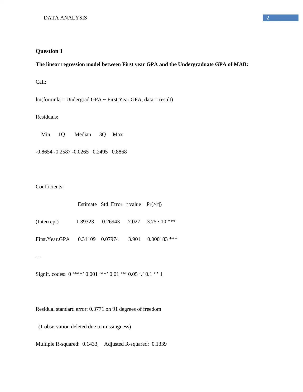
The linear regression model between First year GPA and the Undergraduate GPA of MAB:
Call:
lm(formula = Undergrad.GPA ~ First.Year.GPA, data = result)
Residuals:
Min 1Q Median 3Q Max
-0.8654 -0.2587 -0.0265 0.2495 0.8868
Coefficients:
Estimate Std. Error t value Pr(>|t|)
(Intercept) 1.89323 0.26943 7.027 3.75e-10 ***
First.Year.GPA 0.31109 0.07974 3.901 0.000183 ***
---
Signif. codes: 0 ‘***’ 0.001 ‘**’ 0.01 ‘*’ 0.05 ‘.’ 0.1 ‘ ’ 1
Residual standard error: 0.3771 on 91 degrees of freedom
(1 observation deleted due to missingness)
Multiple R-squared: 0.1433, Adjusted R-squared: 0.1339

DATA ANALYSIS 3
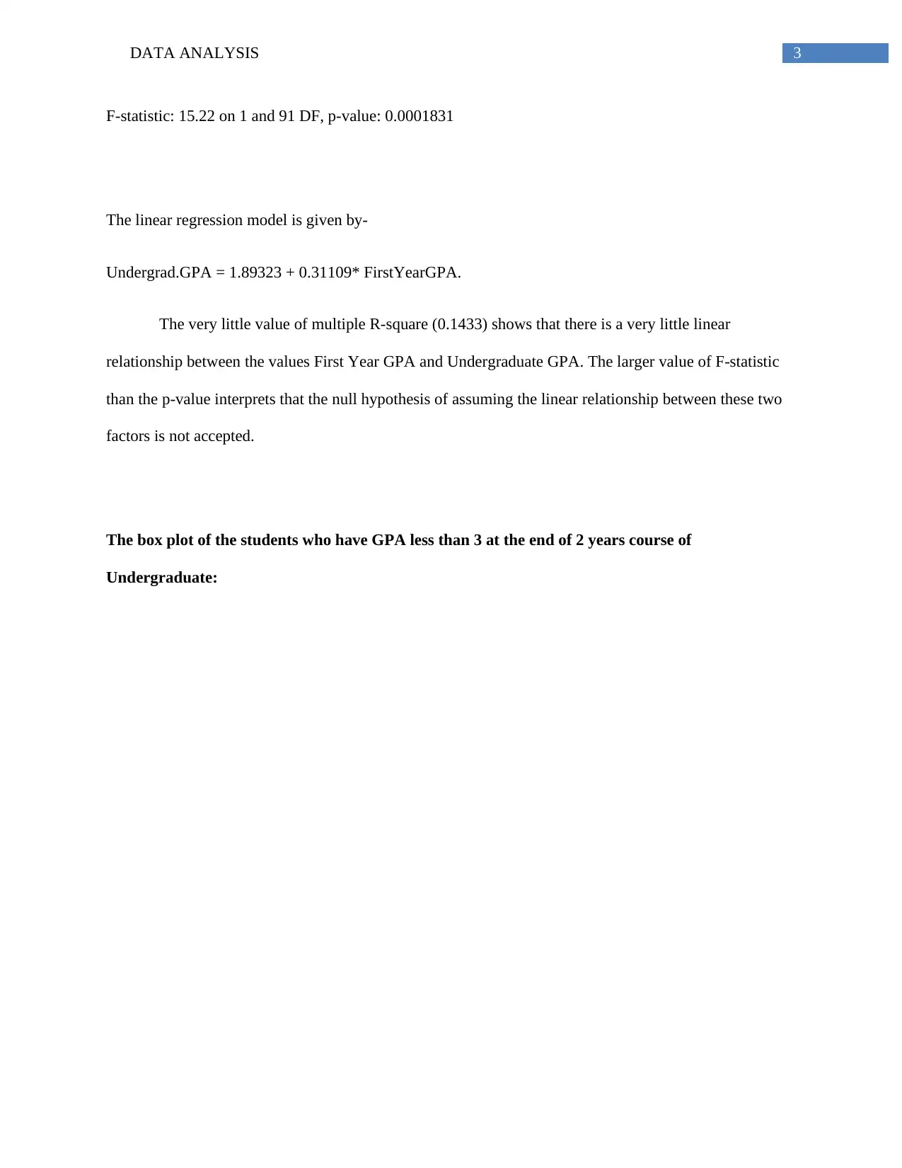
F-statistic: 15.22 on 1 and 91 DF, p-value: 0.0001831
The linear regression model is given by-
Undergrad.GPA = 1.89323 + 0.31109* FirstYearGPA.
The very little value of multiple R-square (0.1433) shows that there is a very little linear
relationship between the values First Year GPA and Undergraduate GPA. The larger value of F-statistic
than the p-value interprets that the null hypothesis of assuming the linear relationship between these two
factors is not accepted.
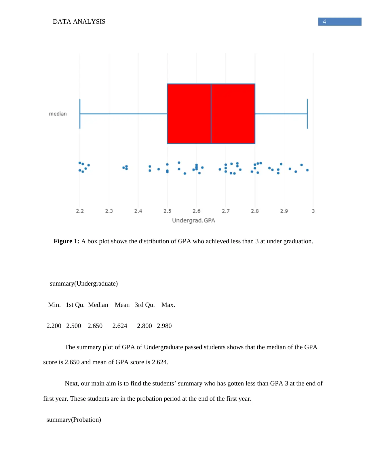
The box plot of the students who have GPA less than 3 at the end of 2 years course of
Undergraduate:

DATA ANALYSIS 4
Figure 1: A box plot shows the distribution of GPA who achieved less than 3 at under graduation.
summary(Undergraduate)
Min. 1st Qu. Median Mean 3rd Qu. Max.
2.200 2.500 2.650 2.624 2.800 2.980
The summary plot of GPA of Undergraduate passed students shows that the median of the GPA
score is 2.650 and mean of GPA score is 2.624.
Next, our main aim is to find the students’ summary who has gotten less than GPA 3 at the end of
first year. These students are in the probation period at the end of the first year.
summary(Probation)

DATA ANALYSIS 5
Min. 1st Qu. Median Mean 3rd Qu. Max.
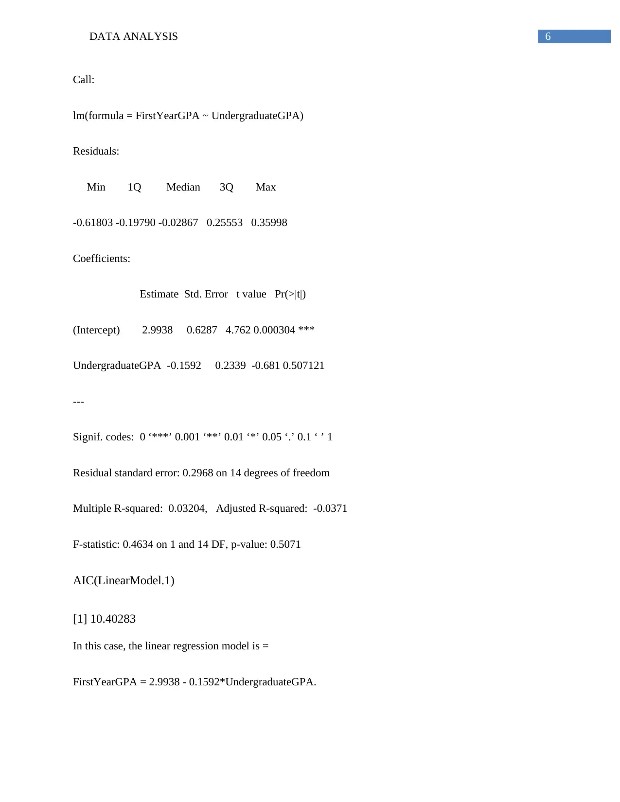
2.000 2.375 2.550 2.569 2.800 2.900
The box plot of the students who have CGPA less at the end of First-year course of MAB program:
Figure 2: A box plot shows the distribution of GPA who achieved less than 3 GPA first year of MAB.
The summary plot of GPA of First Year probationary students shows that the median of the GPA
score is 2.550 and mean of GPA score is 2.569.
The linear regression model shows the linear relationship between the students who were at
probationary after first Year and their GPA after completion of the course:

DATA ANALYSIS 6
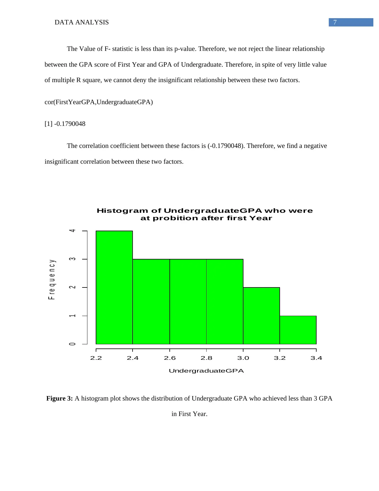
Call:
lm(formula = FirstYearGPA ~ UndergraduateGPA)
Residuals:
Min 1Q Median 3Q Max
-0.61803 -0.19790 -0.02867 0.25553 0.35998
Coefficients:
Estimate Std. Error t value Pr(>|t|)
(Intercept) 2.9938 0.6287 4.762 0.000304 ***
UndergraduateGPA -0.1592 0.2339 -0.681 0.507121
---
Signif. codes: 0 ‘***’ 0.001 ‘**’ 0.01 ‘*’ 0.05 ‘.’ 0.1 ‘ ’ 1
Residual standard error: 0.2968 on 14 degrees of freedom
Multiple R-squared: 0.03204, Adjusted R-squared: -0.0371
F-statistic: 0.4634 on 1 and 14 DF, p-value: 0.5071
AIC(LinearModel.1)
[1] 10.40283
In this case, the linear regression model is =
FirstYearGPA = 2.9938 - 0.1592*UndergraduateGPA.

DATA ANALYSIS 7
The Value of F- statistic is less than its p-value. Therefore, we not reject the linear relationship
between the GPA score of First Year and GPA of Undergraduate. Therefore, in spite of very little value
of multiple R square, we cannot deny the insignificant relationship between these two factors.
cor(FirstYearGPA,UndergraduateGPA)
[1] -0.1790048
The correlation coefficient between these factors is (-0.1790048). Therefore, we find a negative
insignificant correlation between these two factors.
Histogram of UndergraduateGPA who were
at probition after first Year
UndergraduateGPA
F r e q u e n c y
2.2 2.4 2.6 2.8 3.0 3.2 3.4
0 1 2 3 4
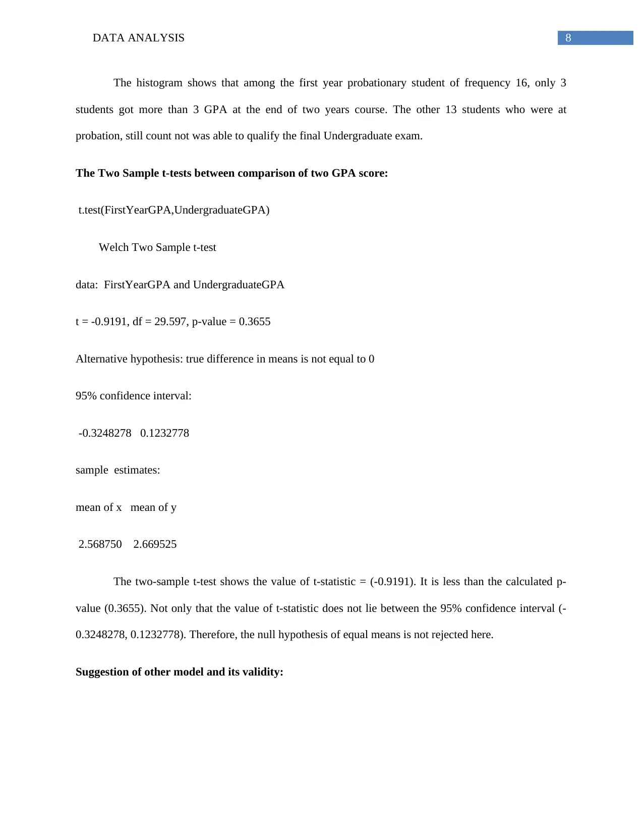
Figure 3: A histogram plot shows the distribution of Undergraduate GPA who achieved less than 3 GPA
in First Year.

DATA ANALYSIS 8
The histogram shows that among the first year probationary student of frequency 16, only 3
students got more than 3 GPA at the end of two years course. The other 13 students who were at
probation, still count not was able to qualify the final Undergraduate exam.
The Two Sample t-tests between comparison of two GPA score:
t.test(FirstYearGPA,UndergraduateGPA)
Welch Two Sample t-test
data: FirstYearGPA and UndergraduateGPA
t = -0.9191, df = 29.597, p-value = 0.3655
Alternative hypothesis: true difference in means is not equal to 0
95% confidence interval:
-0.3248278 0.1232778
sample estimates:
mean of x mean of y
2.568750 2.669525
The two-sample t-test shows the value of t-statistic = (-0.9191). It is less than the calculated p-
value (0.3655). Not only that the value of t-statistic does not lie between the 95% confidence interval (-
0.3248278, 0.1232778). Therefore, the null hypothesis of equal means is not rejected here.
Suggestion of other model and its validity:

DATA ANALYSIS 9
We assumed linear regression model to correlate these factors. Nevertheless, the linear
relationship between these two factors is not properly correlated. We also applied two-sample t-test for
equal mean of GPA of these 2 samples.
Now, if we are interested in applying another statistical model, we can apply multiple regression
models. Here, we cannot apply multiple regression model, because, the two factors are numeric and
discrete in nature.
We cannot use “logit” models also. It is a particular type of multiple regression model because,
the model needs as regressor only categorical and dichotomous variables. In case of Genaralised Linear
Model (GLM), we cannot proceed for singular discrete nature of both the factors. Therefore, inverse
gamma model cannot be implemented here also because, these two factors have no interaction effect.
Lastly, we can proceed to apply Joint Generalised Linear Model (JGLM). This can be a proper
choice of application. We can apply Gamma model or log-linear model to have a better result.
Question 2
Part a)
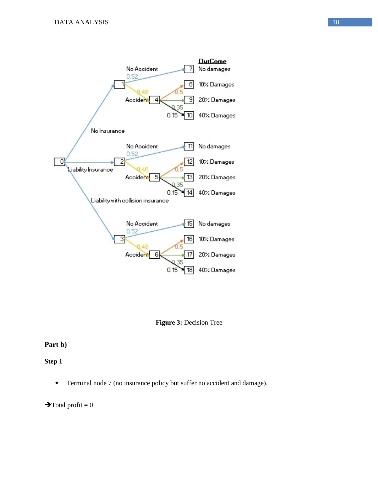
Car chosen for the analysis is Chevrolet Lacetti in Turkey
Book Value = £89390
Turkey’s car accident rate is 48% and no accident is 52%.
The decision tree for the model is given as:

DATA ANALYSIS 10
Figure 3: Decision Tree
Part b)
Step 1
 Terminal node 7 (no insurance policy but suffer no accident and damage).
Total profit = 0

DATA ANALYSIS 11
 Terminal node 8 (no insurance policy but suffer a accident resulting in a damage of 10% of the
car.
Total cost = 0.1(89390) = 8939
Total profit = - 8,939
 Terminal nodes 9 and 10
Total profit for node 9= -17,878
Total profit for node 10 = -35,756
 Terminal node 11 (Liability Insurance policy) costing £670 but suffer no damages.
Total cost = 670
Total profit = -670
 Terminal node 12 (Liability insurance policy) costing £670 but suffer a damage resulting in a loss
of 0.1(89390) = £8939 for which we are reimbursed in full by liability insurance during accident.
Total revenue = 8939
Total cost = 8939 + 670 ; Total profit = -670
From calculation  Reimbursement = Amount Lost (total profit = cost of the insurance).
Same is for terminal nodes 13 and 14 respectively.
Such as a table can be derived as:
Terminal node Total profit £
7 0

DATA ANALYSIS 12
8 -8939
9 -17878
10 -35756
11 -670
12 -670
13 -670
14 -670
15 -450
16 -450-x (x <= 8939)
17 -450-x
18 -450-x
Step 2 - EMV Criterion
As per node 5 on accident, it has branches to terminal nodes 12, 13 and 14.
The monetary value this node comes out to be
0.5(-8939) + 0.35(-17878) + 0.15(-35756) = - 446.95 - 625.73 - 536.34 = -1609.02
EMV for node 1 = 0.52(0) + 0.48(-16090.2) = -7723.296

DATA ANALYSIS 13
EMV for node 2 = -670.
EMV for node 3 = 0.52(-450) + 0.48[0.5(-450-x) + 0.35(-450-x) + 0.15(-450-x)]
= -234 + 0.48(-450-x) = -234 - 0.48x (x <= 8939) = -339.6 as x = -220
Hence at the initial decision node we have the four alternatives
1. No insurance policy EMV = -1609.02
2. Liability Insurance policy EMV = -670
3. Liability with collision insurance policy EMV = -339.6
The best alternative is Liability with collision insurance policy leading an EMV of - £339.6 and the
decision is justified.
Part c)
A policy with deductible at 5% of the car’s value = £4469.5, on a premium of 40%,
Now, Car’s value = 89390 - 4469.5 = 84920.5
If the above scenario is allowed, then the monetary value of node comes out to be
0.5(-8492.05) + 0.35(-16984.1) + 0.15(-33968.2) = - 424.6025 – 594.4435 - 509.523 = -1528.569
The above policy does not define the deductible source as it in increases cost during confidence.
However, when a premium is charged the cost amount to the car owners would be less in comparison. As
a result, a policy deductible would be best for daily wage customers, serviced profession customers or a
customer who is prone to more accidents.

DATA ANALYSIS 14
Part d)
The decision tree has branches and leaves to predictive behavior of variables on different
consideration. The questions devised in decision tree follows a step by step format in which questions are
dependent on answers to the previous questions of the sequence. Simulation can be more confusing
because decisions are modeled as rules and used with common statistical distributions whereas a decision
tree assesses the probability values because it can be calculated and can be shown in a tree. Also, in
simulation results do not become stable as they are independent but in decision tree portions are
meaningful and understanding. Also, decision tree is much more helpful than simulation because
“strategy map” is made for decisions and values going forward.

DATA ANALYSIS 15
Bibliography:
Clemen, R.T. and Reilly, T., 2013. Making hard decisions with DecisionTools. Cengage Learning.
Draper, N.R. and Smith, H., 2014. Applied regression analysis. John Wiley & Sons.
Eiselt, H.A. and Sandblom, C.L., 2012. Decision Analysis. In Operations Research (pp. 303-331).
Springer Berlin Heidelberg.
Fox, J., 2015. Applied regression analysis and generalized linear models. Sage Publications.
Kleinbaum, D., Kupper, L., Nizam, A. and Rosenberg, E., 2013. Applied regression analysis and other
multivariable methods. Nelson Education.
Montgomery, D.C., 2017. Design and analysis of experiments. John Wiley & Sons.
Ott, R.L. and Longnecker, M.T., 2015. An introduction to statistical methods and data analysis. Nelson
Education.
Turner, R.M., Jackson, D., Wei, Y., Thompson, S.G. and Higgins, J., 2015. Predictive distributions for
between‐study heterogeneity and simple methods for their application in Bayesian meta‐
analysis. Statistics in medicine, 34(6), pp.984-998.