Data Analysis and Forecasting

This study material covers various topics related to data analysis and forecasting. It explains the concepts of mean, mode, median, range, and standard deviation. It also discusses linear forecasting models. The material provides insights into making informed decisions using data analysis techniques.

Data Analysis and
Forecasting

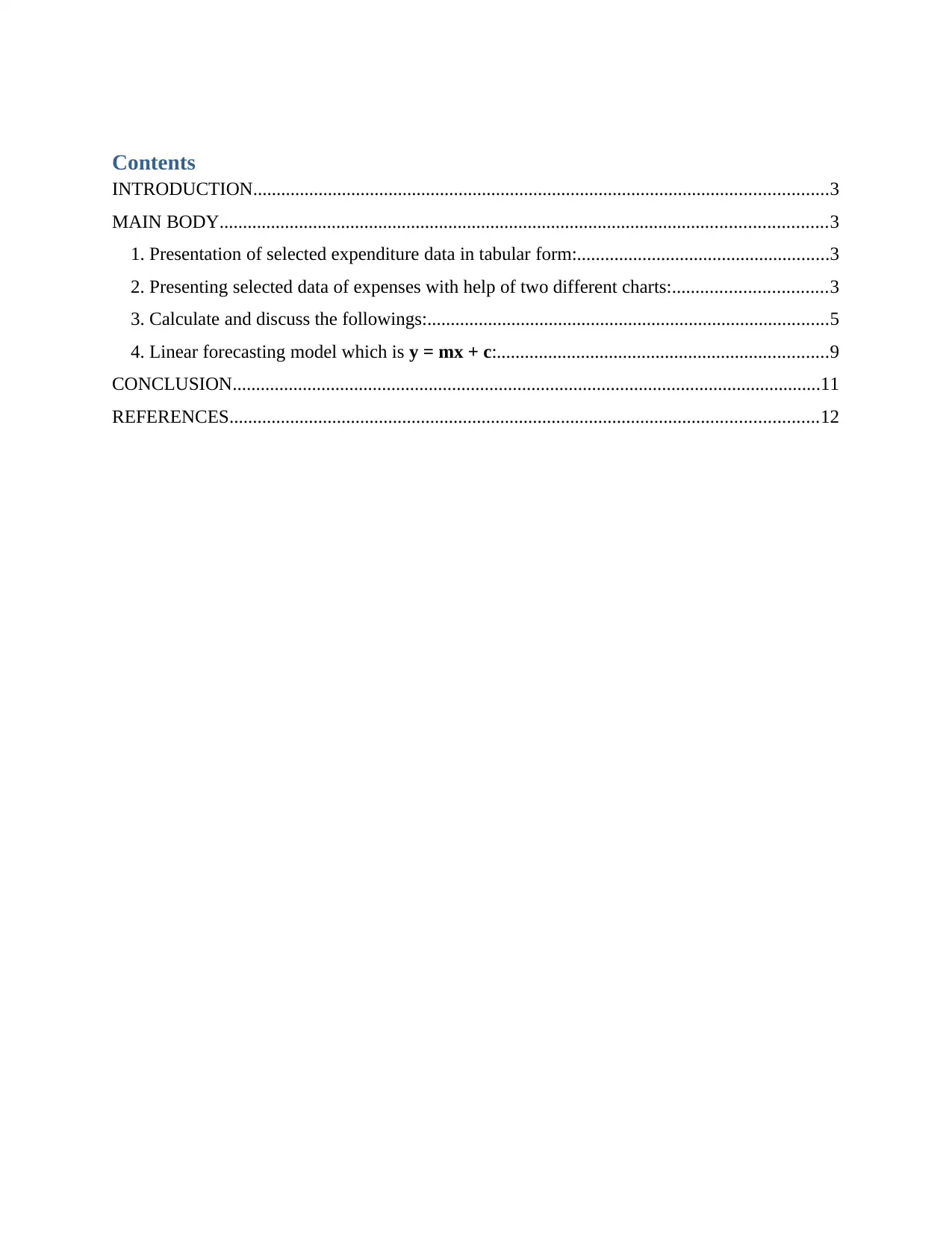
Contents
INTRODUCTION...........................................................................................................................3
MAIN BODY..................................................................................................................................3
1. Presentation of selected expenditure data in tabular form:......................................................3
2. Presenting selected data of expenses with help of two different charts:.................................3
3. Calculate and discuss the followings:......................................................................................5
4. Linear forecasting model which is y = mx + c:.......................................................................9
CONCLUSION..............................................................................................................................11
REFERENCES..............................................................................................................................12

INTRODUCTION
Data analysis alludes to the system of statistical analysis, review, transfer, and retrieval
that seeks to discover key findings of knowledge informing and assisting in decisions.
Mechanisms of the data analysis have common attributes and procedures, below the number of
categories containing several strategies, and are used in different fields of industry, findings,
and mathematics. In present business ecosystem data analysis performs a key part in making
more informed decisions and aiding organizations to operate more effectively (Miles, Huberman
and Saldaña, 2018). With 10 sequential months’ expenditures data, the study-assessment discuss
about various data analysis-related topics such as standard deviation, mean model, median value,
mode etc. Furthermore, the assessment covers linear forecasting approach for estimating
expenditures for eleventh and twelfth months.
MAIN BODY
1. Presentation of selected expenditure data in tabular form:
Mont
h
Month-
wise
Expense
s
Jan 1500
Feb 2100
Marc
h 1400
April 1900
May 1800
June 1700
July 1700
Aug 1500
Sep 1600
Oct 2000

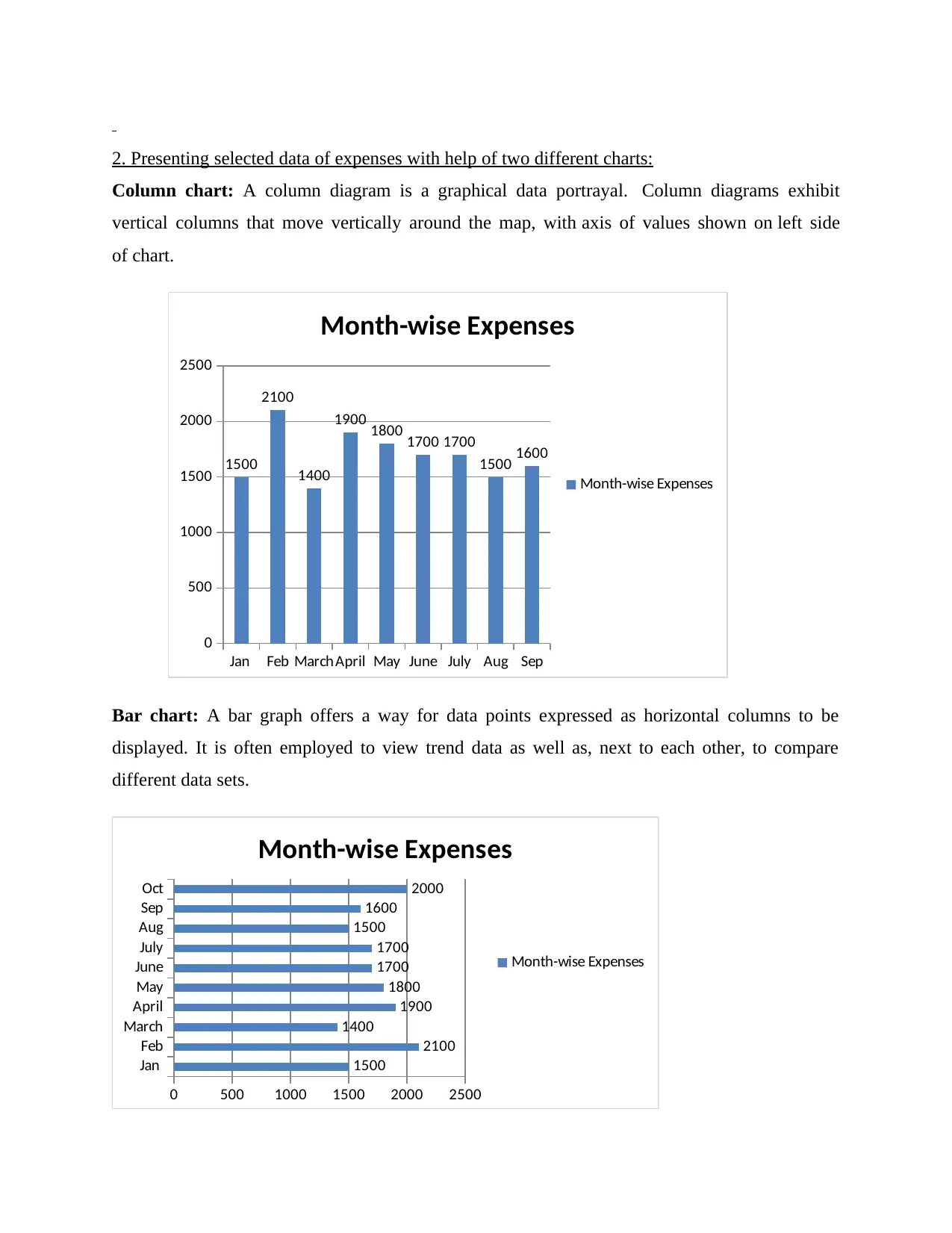
2. Presenting selected data of expenses with help of two different charts:
Column chart: A column diagram is a graphical data portrayal. Column diagrams exhibit
vertical columns that move vertically around the map, with axis of values shown on left side
of chart.
Jan Feb MarchApril May June July Aug Sep
0
500
1000
1500
2000
2500
1500
2100
1400
1900 1800 1700 1700
1500 1600
Month-wise Expenses
Month-wise Expenses
Bar chart: A bar graph offers a way for data points expressed as horizontal columns to be
displayed. It is often employed to view trend data as well as, next to each other, to compare
different data sets.
Jan
Feb
March
April
May
June
July
Aug
Sep
Oct
0 500 1000 1500 2000 2500
1500
2100
1400
1900
1800
1700
1700
1500
1600
2000
Month-wise Expenses
Month-wise Expenses

3. Calculate and discuss the followings:
Mean: The mean figure represents the total average of given number: center value of calculated
number set. That is, it is average value in fundamental facets. This is quite meaningful, though it
requires most of the calculations to figure out. Analyses of central tendency or mean are utilized
in variety of ways as well as represent the base of statistical data. The equation for assessing the
average is proportion of sum of selected values to no. of observations (Saidi and Siew, 2019).
Month Month-wise Expenses
Jan 1500
Feb 2100
March 1400
April 1900
May 1800
June 1700
July 1700
Aug 1500
Sep 1600
Oct 2000
Aggregate or Σx 17200
Mean = Σx / n
= 17200 / 10
= 1720
Mode: This is the most frequent or predominant point of the distributions, which is value X
referring to the highest point of the distribution. The larger frequency distribution here is

considered to be multi-faceted when larger than 1 shares and will be described by increases at
two different levels in distributions.
Mont
h
Month-
wise
Expense
s
Jan 1500
Feb 2100
Marc
h 1400
April 1900
May 1800
June 1700
July 1700
Aug 1500
Sep 1600
Oct 2000
On the bases of the stated table and coloured rows, this has been measured that here 1700 is most
frequently appearing value in identified numbers that is two times. Thus for data, mode would be
1720.
Median- Median refers to the score that divides the total distribution two equal parts; half of the
points are beyond median when data are arranged as in quantitative series, and almost half (50
percent) are well below that. That is central attribute which may be advantageous if there is an
extremely greater or lesser value in compilation of figures. In distribution, the median is often
linked to as the 50th percentile value. The equation (N+1)/2 may be utilized to locate N figures
within median position. Thus, when N being odd no., the formula generates attribute that
encompasses value in numerically ordered distribution referring to the median position (Kaur,
Stoltzfus and Yellapu, 2018).

If Odd values, then the Median = (N+1)/2th item.
If Even values, then Median ={N/2th item+ N/2th item + 1)/2
In study dataset has even number which is ten so major steps for assessing median are, as
follows:
Arranging given data in the ascending order:
Mont
h
Month-
wise
Expense
s (x)
Marc
h 1400
Jan 1500
Aug 1500
Sep 1600
June 1700
July 1700
May 1800
April 1900
Oct 2000
Feb 2100
N= 10
M= (10/2th item + 10/2th item + 1)/2
= (5th item+ 6th item)/2
= (1700 + 1700)/2
= 3500 / 2

= 1700
Range: Range is the contrast among the highest and the lowest value of the distribution. It's not
commonly considered as sole measure of variability because this focuses solely on the most
extreme points of distributions and doesn't reflect trend of variability in the distribution.
Higher value = 2100
Lower value = 1400
Range= (2100 - 1400)
= 700
Standard deviation: Standard deviation delivers insights into the degree of variation within a
collection of parameters (average). Standard deviation figure is positive value of square-root of
the variance. Variance of the square quantities is proportional and has marginal meaning with
respect to the outcomes The SD is thus the measurement of variability expressed in same
value as data (Rousselet and Wilcox, 2020).
Month Month-
wise
Expenses
(x)
x-
mean
(x-
mean)2
Jan 1500 -220 48400
Feb 2100 380 144400
March 1400 -320 102400
April 1900 180 32400
May 1800 80 6400
June 1700 -20 400
July 1700 -20 400
Aug 1500 -220 48400
Sep 1600 -120 14400
Oct 2000 280 78400

∑x = 17200 ∑(x –
mean) 2
=
476000
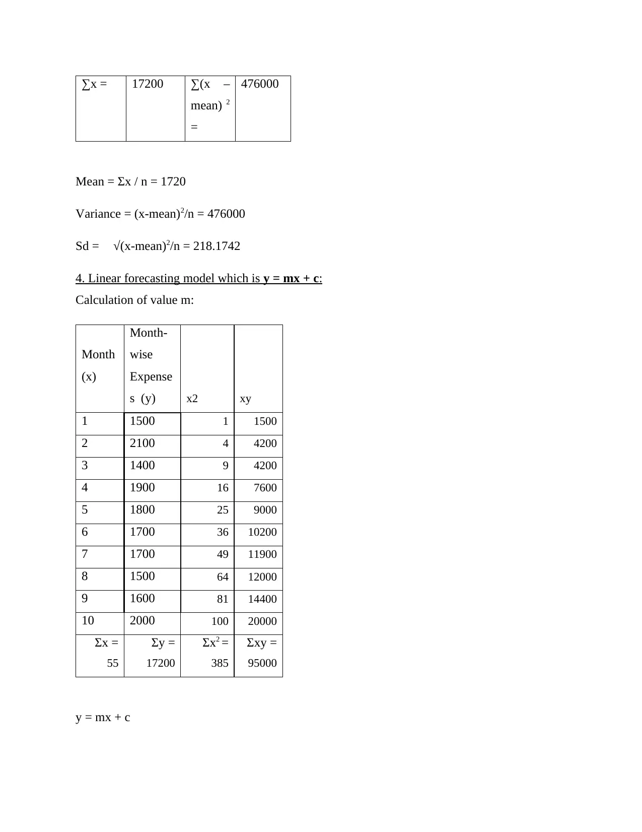
Mean = Σx / n = 1720
Variance = (x-mean)2/n = 476000
Sd = √(x-mean)2/n = 218.1742
4. Linear forecasting model which is y = mx + c:
Calculation of value m:
Month
(x)
Month-
wise
Expense
s (y) x2 xy
1 1500 1 1500
2 2100 4 4200
3 1400 9 4200
4 1900 16 7600
5 1800 25 9000
6 1700 36 10200
7 1700 49 11900
8 1500 64 12000
9 1600 81 14400
10 2000 100 20000
Σx =
55
Σy =
17200
Σx2 =
385
Σxy =
95000
y = mx + c

Here,
m=
n (∑xy) - (∑x) (∑y)/ n(∑x2)-( ∑x)2
= 10*(95000)-(55)*(17200)/10*(385)-(55)2
= 950000 - 946000/3850-3025
= 4000/825
= 4.8485
Calculation of c:
c = [(∑y) / n]-m (∑x/n)
= [17200/10]- 4.8485 (55/10)
= 1720-26.66667
= 1713.33
Forecasting for month 11 and 12:
Forecasting for month 11:
y = mx+c
= 4.8485 * 11 + 1713.33
= 1766.66 OR 1767

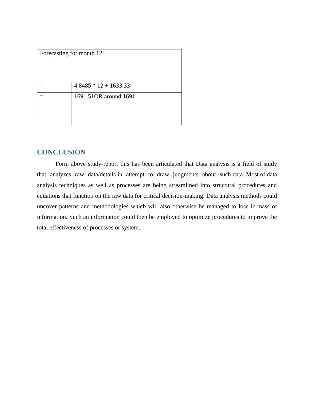
Forecasting for month 12:
= 4.8485 * 12 + 1633.33
= 1691.51OR around 1691
CONCLUSION
Form above study-report this has been articulated that Data analysis is a field of study
that analyzes raw data/details in attempt to draw judgments about such data. Most of data
analysis techniques as well as processes are being streamlined into structural procedures and
equations that function on the raw data for critical decision-making. Data analysis methods could
uncover patterns and methodologies which will also otherwise be managed to lose in mass of
information. Such an information could then be employed to optimize procedures to improve the
total effectiveness of processes or system.

REFERENCES
Books and Journal:
Miles, M.B., Huberman, A.M. and Saldaña, J., 2018. Qualitative data analysis: A methods
sourcebook. Sage publications.
Saidi, S.S. and Siew, N.M., 2019. Assessing Students' Understanding of the Measures of Central
Tendency and Attitude towards Statistics in Rural Secondary Schools. International
Electronic Journal of Mathematics Education, 14(1), pp.73-86.
Kaur, P., Stoltzfus, J. and Yellapu, V., 2018. Descriptive statistics. International Journal of
Academic Medicine, 4(1), p.60.
Rousselet, G.A. and Wilcox, R.R., 2020. Reaction times and other skewed distributions:
problems with the mean and the median. Meta-Psychology, 4.