Analysis of Average Hourly Earnings and Housing Trends

This assignment delves into the analysis of average hourly earnings, investigating factors like age, gender, and education level to determine their influence on earnings. The report also examines housing trends in Sydney, Australia, focusing on interest rates, principal amounts, and year-over-year changes. Additionally, it explores the portfolio ratio as a key metric for financial analysis.

Running head: DATA ANALYSIS OF ECONOMETRICS
Data Analysis of Econometrics
Name of the University:
Name of the Student:
Author’s Note:

DATA ANALYSIS OF ECONOMETRICS 1
Executive Summary:
The report describes economic skills with the help of regression analysis. We answered three
questions and their subparts. We have provided the necessary calculations and tables. We
interpreted from the analysis with the help of MS Office, Minitab and R. We finally have
drawn the conclusions from each question.

DATA ANALYSIS OF ECONOMETRICS 2
Table of Contents
Introduction:...............................................................................................................................3
Questions and Answers:.............................................................................................................3
Question A.............................................................................................................................3
Question B..............................................................................................................................6
Question C............................................................................................................................23
Conclusion:..............................................................................................................................29
Bibliography List:....................................................................................................................30

DATA ANALYSIS OF ECONOMETRICS 3
Introduction:
We described here the group-survey of Australian data of different cities. The answers
of three questions are provided in the analysis. We derived the comparative study of different
Australian cities in the first part. In the second part, we calculated the analysis of economic
situation and relation of chosen three sectors. In the third part, we analyzed the data of age,
average hourly earnings and different factors.
We have elaborately analyzed the dataset with the help of MS Office, Minitab and R.
We installed add-ins in MS excel for advance analysis (Slazek et al. 2013). The report would
help the economic investigators of Australia.
Data analysis on econometrics in this report shows the overview of three different
segments of economics in this report.
Questions and Answers:
Question A (Australian House Price Index):
A1.

DATA ANALYSIS OF ECONOMETRICS 4
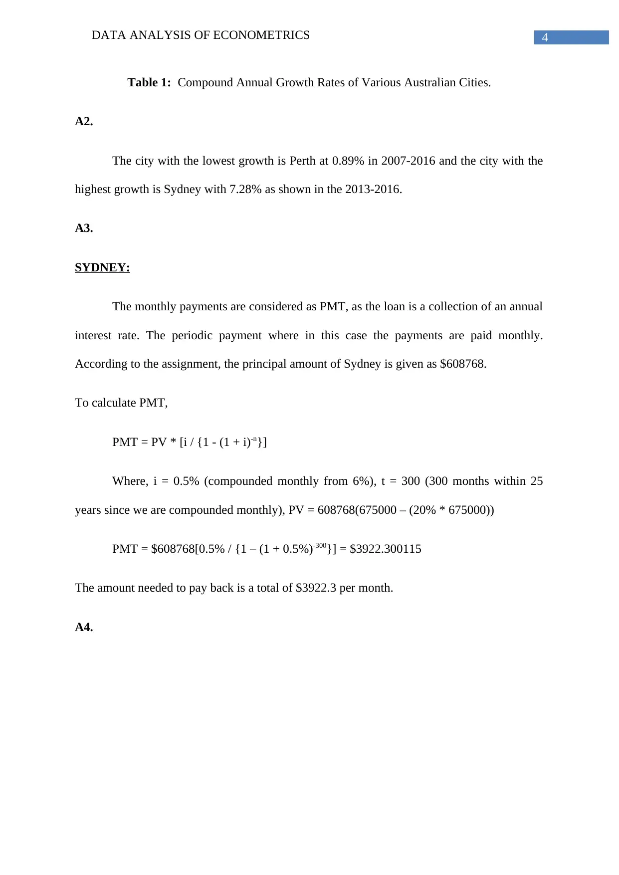
Table 1: Compound Annual Growth Rates of Various Australian Cities.
A2.
The city with the lowest growth is Perth at 0.89% in 2007-2016 and the city with the
highest growth is Sydney with 7.28% as shown in the 2013-2016.
A3.
SYDNEY:
The monthly payments are considered as PMT, as the loan is a collection of an annual
interest rate. The periodic payment where in this case the payments are paid monthly.
According to the assignment, the principal amount of Sydney is given as $608768.
To calculate PMT,
PMT = PV * [i / {1 - (1 + i)-n}]
Where, i = 0.5% (compounded monthly from 6%), t = 300 (300 months within 25
years since we are compounded monthly), PV = 608768(675000 – (20% * 675000))
PMT = $608768[0.5% / {1 – (1 + 0.5%)-300}] = $3922.300115
The amount needed to pay back is a total of $3922.3 per month.
A4.

DATA ANALYSIS OF ECONOMETRICS 5
1
3
5
7
9
11
13
15
17
19
21
23
25
27
29
31
33
0%
10%
20%
30%
40%
50%
60%
70%
80%
90%
100%
Principal Amount
Interest Amount of SYDNEY
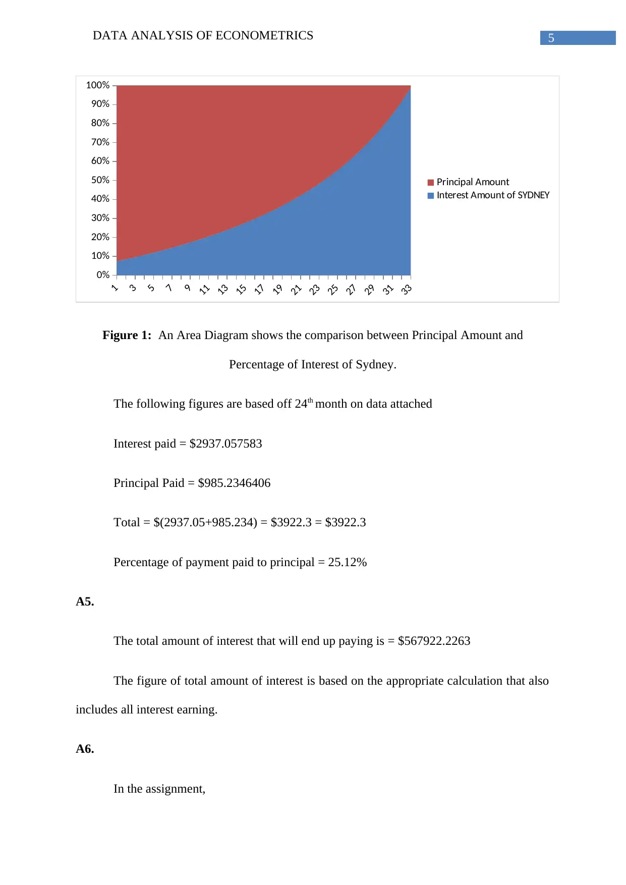
Figure 1: An Area Diagram shows the comparison between Principal Amount and
Percentage of Interest of Sydney.
The following figures are based off 24th month on data attached
Interest paid = $2937.057583
Principal Paid = $985.2346406
Total = $(2937.05+985.234) = $3922.3 = $3922.3
Percentage of payment paid to principal = 25.12%
A5.
The total amount of interest that will end up paying is = $567922.2263
The figure of total amount of interest is based on the appropriate calculation that also
includes all interest earning.
A6.
In the assignment,

DATA ANALYSIS OF ECONOMETRICS 6
Sydney House Price: $675000
CAGR: 5.05%
Year 25: FV = Current Value*(1+r) n = 675000(1+5.05%) 25 = $2314128.793
House Appreciation = Future Value of House Price – Current Value of House Price
= 2314128.793 – 675000 = $1639128.793
As, $1639128.793 > $567922.2263; Therefore, we can say that, House Appreciation
> Total Interest Paid.
From our above calculation, we can conclude that the value of the house is greater
than the interest paid thus the value appreciation is sufficient to cover the total interest paid.
Question B.
The three chosen securities are industrial in Mix. And Fix., consumer services in
travel and tourism and healthcare providers. The value of ri in the industrial, consumer
services and Healthcare services are calculated separately.
B1.
A. Orthogonal Least Square (OLS) model of Adelaide Brighton (Market Value and
Stock Value):

DATA ANALYSIS OF ECONOMETRICS 7
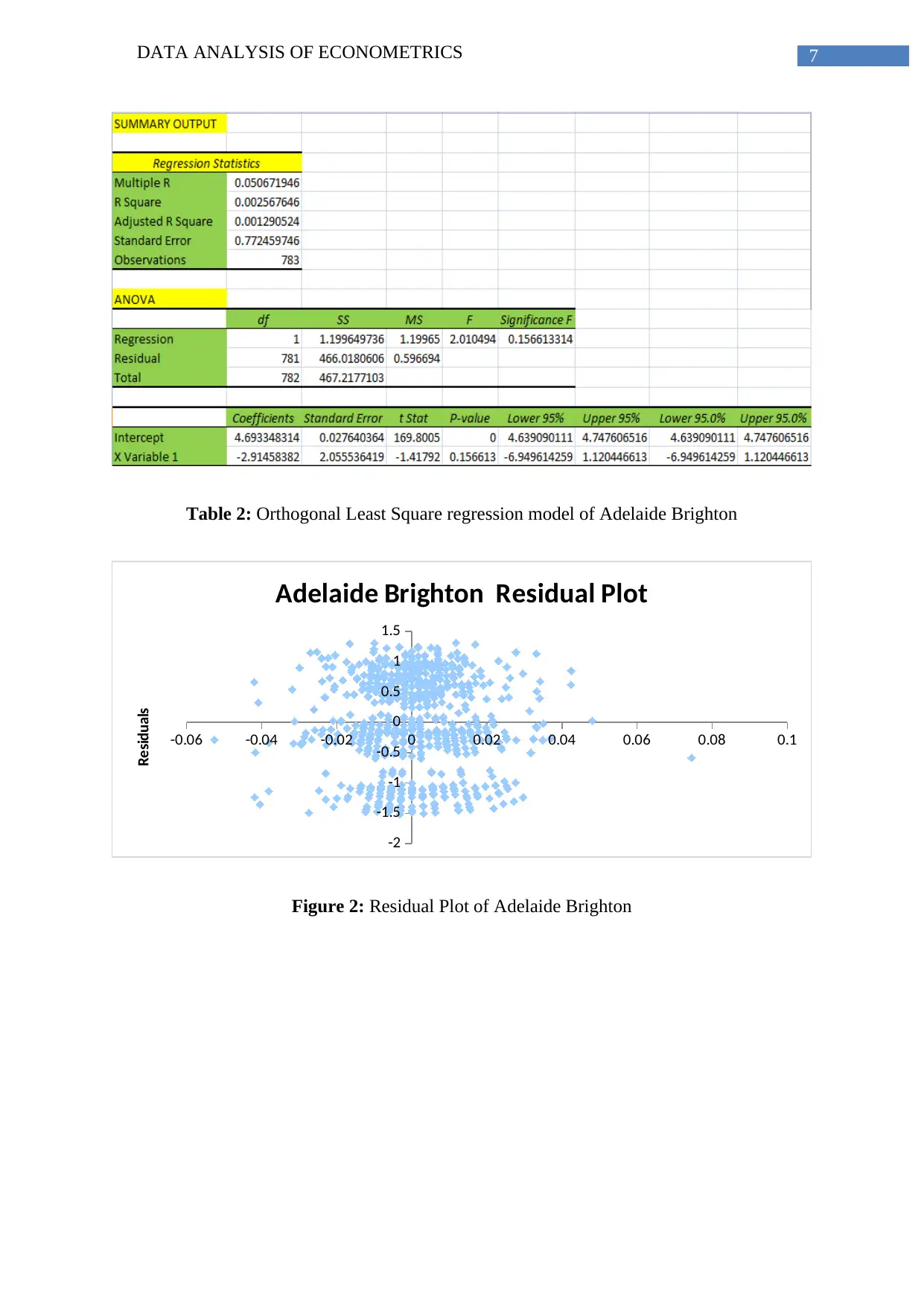
Table 2: Orthogonal Least Square regression model of Adelaide Brighton
-0.06 -0.04 -0.02 0 0.02 0.04 0.06 0.08 0.1
-2
-1.5
-1
-0.5
0
0.5
1
1.5
Adelaide Brighton Residual Plot
Residuals
Figure 2: Residual Plot of Adelaide Brighton

DATA ANALYSIS OF ECONOMETRICS 8
0.005617978 0.024657534 0 0.005847953 0.033268102 0.014035088
0
1
2
3
4
5
6
7
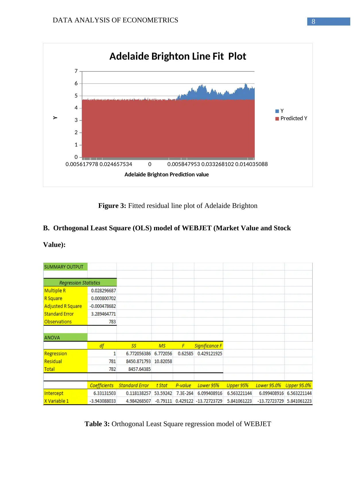
Adelaide Brighton Line Fit Plot
Y
Predicted Y
Adelaide Brighton Prediction value
Y
Figure 3: Fitted residual line plot of Adelaide Brighton
B. Orthogonal Least Square (OLS) model of WEBJET (Market Value and Stock
Value):
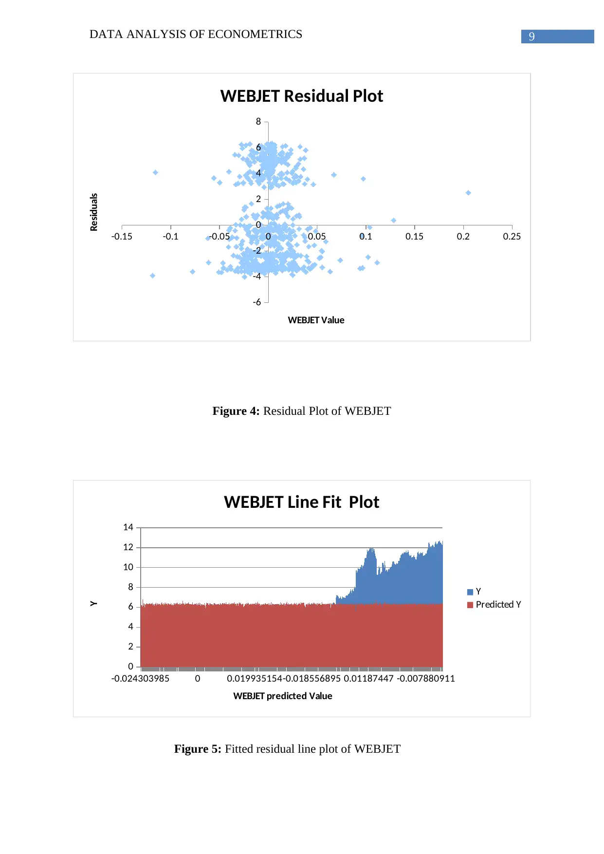
Table 3: Orthogonal Least Square regression model of WEBJET

DATA ANALYSIS OF ECONOMETRICS 9
-0.15 -0.1 -0.05 0 0.05 0.1 0.15 0.2 0.25
-6
-4
-2
0
2
4
6
8
WEBJET Residual Plot
WEBJET Value
Residuals
Figure 4: Residual Plot of WEBJET
-0.024303985 0 0.019935154-0.018556895 0.01187447 -0.007880911
0
2
4
6
8
10
12
14
WEBJET Line Fit Plot
Y
Predicted Y
WEBJET predicted Value
Y
Figure 5: Fitted residual line plot of WEBJET

DATA ANALYSIS OF ECONOMETRICS 10
C. Orthogonal Least Square (OLS) model of RAMSEY Healthcare (Market Value and
Stock Value):
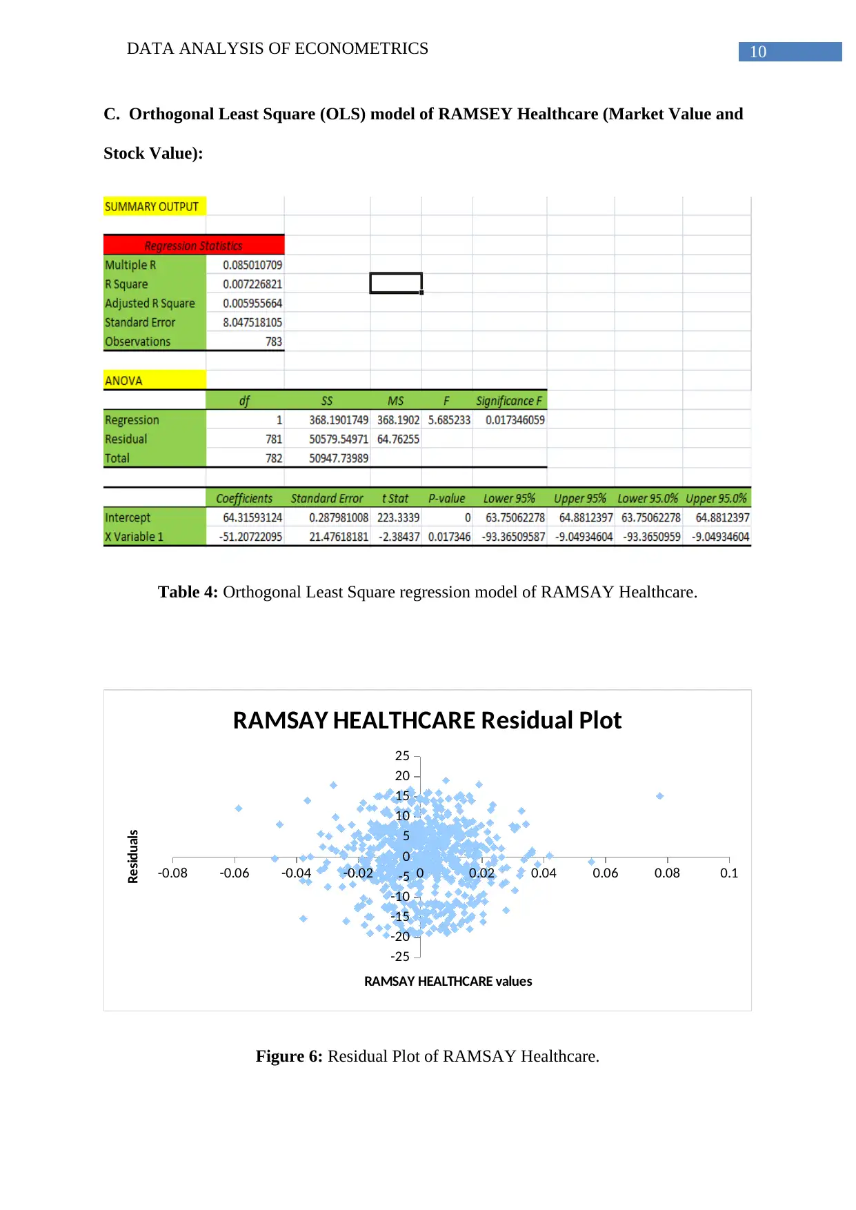
Table 4: Orthogonal Least Square regression model of RAMSAY Healthcare.
-0.08 -0.06 -0.04 -0.02 0 0.02 0.04 0.06 0.08 0.1
-25
-20
-15
-10
-5
0
5
10
15
20
25
RAMSAY HEALTHCARE Residual Plot
RAMSAY HEALTHCARE values
Residuals
Figure 6: Residual Plot of RAMSAY Healthcare.

DATA ANALYSIS OF ECONOMETRICS 11
0.011123228 0.012152489 -0.012295772 0.015063168 0.016322404 0.008878128
0
10
20
30
40
50
60
70
80
90
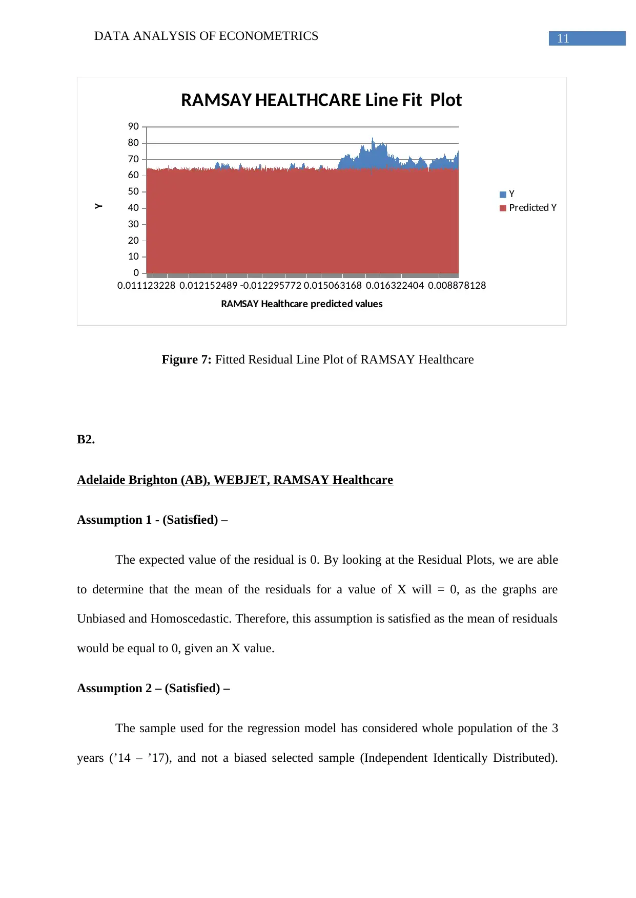
RAMSAY HEALTHCARE Line Fit Plot
Y
Predicted Y
RAMSAY Healthcare predicted values
Y
Figure 7: Fitted Residual Line Plot of RAMSAY Healthcare
B2.
Adelaide Brighton (AB), WEBJET, RAMSAY Healthcare
Assumption 1 - (Satisfied) –
The expected value of the residual is 0. By looking at the Residual Plots, we are able
to determine that the mean of the residuals for a value of X will = 0, as the graphs are
Unbiased and Homoscedastic. Therefore, this assumption is satisfied as the mean of residuals
would be equal to 0, given an X value.
Assumption 2 – (Satisfied) –
The sample used for the regression model has considered whole population of the 3
years (’14 – ’17), and not a biased selected sample (Independent Identically Distributed).

DATA ANALYSIS OF ECONOMETRICS 12
Further, as each daily return does not affect any other daily returns, they are independent to
each other. Therefore, this assumption is satisfied as the selected data is IID.
Assumption 3 – (Satisfied) –
It can be determined that there are no outliers, which can be determined by inspecting
the line fit plot. Since, there are no outliers which can be determined by inspecting the line fit
plot, since there are no outliers it can be concluded in a meaningless value of an estimated
“Beta 1”, in which this assumption is satisfied.
Assumption 4 – (Satisfied) –
The error term has a zero-conditional mean. In other words, each stock OLS specifies
each linear model such that there are no omitted variables.
Assumption 5 – (Satisfied) –
The error term (e) is constant across all stocks. They all remain with the same
variance and are not correlated with each other in anyway. This is known to be in a state of
homoscedasticity.
B3.
Beta Values
The beta values are calculated from the coefficient of the ASX 200 market return
independent variable from the regression. The three estimated betas (slopes) from three
stocks are respectively (-2.92) (industrial), (-3.94) (consumer services), (-51.07) (healthcare
providers).
The betas do not line as our expectation. The reason is that the market and stock
factors are not properly linearly related.

DATA ANALYSIS OF ECONOMETRICS 13
Adelaide Brighton:
The beta is -2.92. This beta is in line with our expectation for the following reasons:
1. The Adelaide Brighton stock is more volatile than the market and contains higher
risk compared to the other two stocks mainly due to its market capitalization.
2. Adelaide Brighton has a large weighting of close to 9% of the ASX 200 relating to
market capitalization and therefore its performance would be closely correlated to
the ASX 200 performance.
Statistical Significance
H0: β ̂ market=0. If there is a low p-value or high-test statistic (t-stat), then we
reject the null. Here the P-Value is 0.15663 >0.05, which implies that the critical
value does not lie within the rejection region. Therefore, we cannot reject the null
hypothesis. These statistics indicate that the market does have a statistically
significant impact on the returns of Adelaide Brighton.
WEBJET
The Beta of WEBJET is (-3.94).This Beta is in line with our expectations for the
following reasons:
1. WEBJET is a market leader in the Airlines industry. As the demand for Airlines
will be stable it is less volatile than the market, hence has minimal risk. Another
influencing factor in this is that the industry is not as competitive as the other
comparing stocks contributing to the stability of the beta.

DATA ANALYSIS OF ECONOMETRICS 14
2. Thus, WEBJET’s business will also be stable and more resilient to market shocks.
3. WEBJET is an Australian company and therefore it will still have some
correlation with the market risk and therefore we would not expect a beta close to
0.
Statistical Significance
H0: β ̂ market = 0. If there is a low p-value or high-test statistic (t-stat), then we
reject the null. For WEBJET, the P-Value is 0.429 > 0.05, which implies that the
critical value does not lie within the rejection region. Therefore, we cannot reject
the null hypothesis. These statistics indicate that the market statistically significant
impact on the returns of WEBJET.
RAMSAY Healthcare
The Beta of Ramsay Healthcare is (-51.207). The volatility is minimal and so is
the risk. This is maybe contributed by the industry, which Ramsay Healthcare is in,
where the competition is tolerable.
1. Ramsay Healthcare lies within the pharmaceutical sector where the primary
factor in return is the sales of it’s products. Thus, compared to other stocks in the
ASX200 the volatility is minimal and so is the risk.
2. The primary factor affecting RAMSAY Healthcare's consumption of its
products and public’s view is its services. Therefore, it has higher than the market that
is demonstrated by its beta being > 1.
3. Ramsay Healthcare is an Australian company and therefore it will still have
some correlation with the market risk and therefore we would not expect a beta close
to 0.

DATA ANALYSIS OF ECONOMETRICS 15
Statistical Significance
1. H0: β ̂ market=0. If there is a low p-value or high-test statistic (t-stat), then we
reject the null. For Ramsay Industries, the P-Value is 0.0173 < 0.05, which
implies that the critical value does lie within the rejection region. Therefore, we
can reject the null hypothesis. These statistics indicate that the market does have a
statistically significant impact on the returns of Ramsay Industries.
2. All three betas are mostly in line with our expectations due to their characteristics
within the market. However, we expected Ramsay Healthcare’s beta to be closer
to 1 due to the fact that they are market leaders within their industry.
3. Beta is the measure of the stock’s volatility in relation to the market. The market
is considered to have a beta of 1 and stocks are ranked based on how much they
deviate from the market. Stocks with a beta of less than 1 are less volatile than the
market and stocks with a beta of more than 1 are more volatile. Zero beta stocks
have zero correlation with market movements. They are expected to have a low
risk free returns.
Beta Equal to One: The Beta which is the level of risk of the market is considered = 1
and is called "Systematic Risk". If a stock has a Beta = 1, it therefore has the same
risk level as the market. If the market moves by 1 point, the stock should also reflect
this movement by 1 unit.
Beta Equal to Zero: A zero Beta stock implies that is has no "Systematic Risk", and
would be considered a "Risk- Free" rate. Further, this would imply that the return on
this stock will has no correlation with the market. This can be seen through regression
analysis as the coefficient of an independent variable (Beta) would be multiplied by 0,
and therefore would not impact the dependent variable i.e. Return.

DATA ANALYSIS OF ECONOMETRICS 16
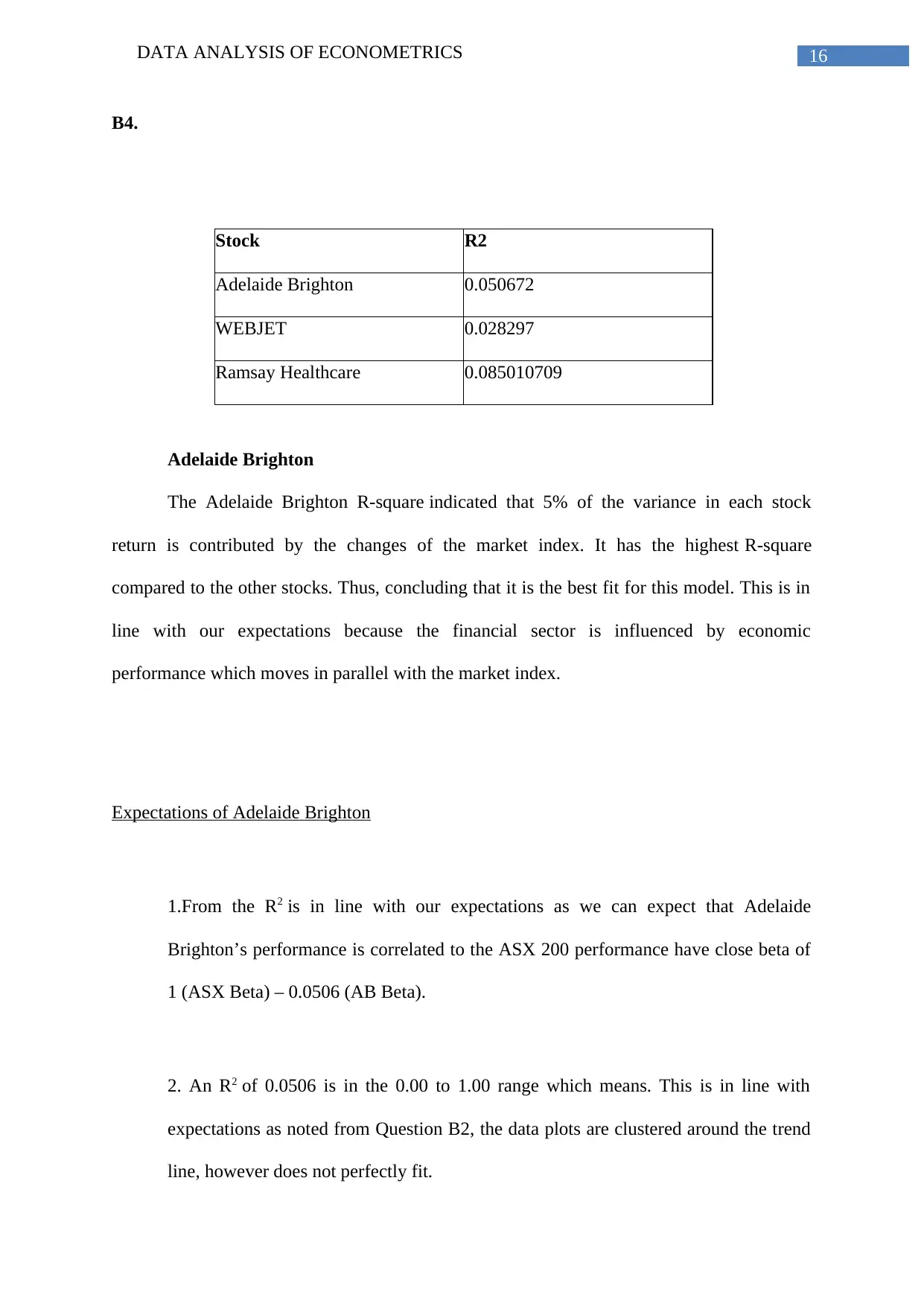
B4.
Stock R2
Adelaide Brighton 0.050672
WEBJET 0.028297
Ramsay Healthcare 0.085010709
Adelaide Brighton
The Adelaide Brighton R-square indicated that 5% of the variance in each stock
return is contributed by the changes of the market index. It has the highest R-square
compared to the other stocks. Thus, concluding that it is the best fit for this model. This is in
line with our expectations because the financial sector is influenced by economic
performance which moves in parallel with the market index.
Expectations of Adelaide Brighton
1.From the R2 is in line with our expectations as we can expect that Adelaide
Brighton’s performance is correlated to the ASX 200 performance have close beta of
1 (ASX Beta) – 0.0506 (AB Beta).
2. An R2 of 0.0506 is in the 0.00 to 1.00 range which means. This is in line with
expectations as noted from Question B2, the data plots are clustered around the trend
line, however does not perfectly fit.

DATA ANALYSIS OF ECONOMETRICS 17
WEBJET
The WEBJET R2 indicated that 2.829% of the variance in the stock return is
correlated to the market index. This can be justified by the characteristics of the stock
within the market due to its low competitive forces in a stable market.
Expectations of WEBJET
1. From the R2 is in line with our expectations as we can expect that
WEBJET’s performance is correlated to the ASX 200 performance have close beta of
1 (ASX Beta) – 0.02829 (WEBJET)
2.An R2 of 0.02829 is in the 0.00 to 1.00 range. This is in line with
expectations as noted from Question B2, the data plots are clustered around the trend
line, however does not perfectly fit.
RAMSAY Healthcare:
The Ramsay Healthcare R2 indicated that 8.053% of the variance in the stock return
is associated to the market index. This is the lowest measure of fit out of the three
stocks that is not in line with our expectations. Similar to the comment made in B2 for
the beta, we expected Ramsay Healthcare’s R2 to be higher because they are market
leaders within their industry.

DATA ANALYSIS OF ECONOMETRICS 18
Expectations of CCL
1.From the R2 is in line with our expectations as we can expect that Ramsay
Healthcare’s performance is correlated to the ASX 200 performance have close beta
of 1 (ASX Beta) – 0.08053 (Ramsay Beta)
2. An R2 of 0.08053 is in the 0.00 to 1.00 range. This is in line with expectations as
noted from Question B2, the data plots are clustered around the trend line, however
does not perfectly fit (Ott and Longnecker 2015).
B5.
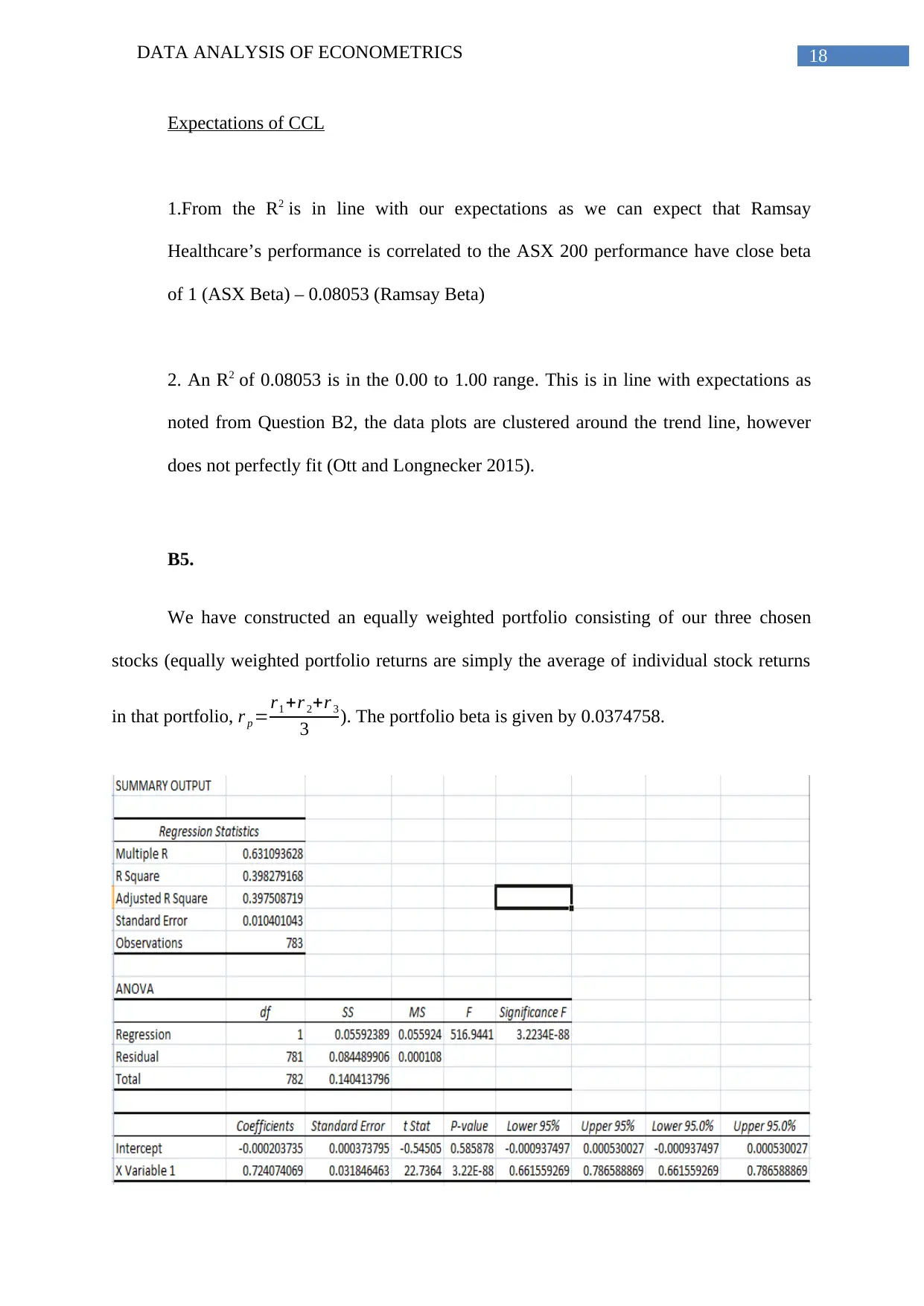
We have constructed an equally weighted portfolio consisting of our three chosen
stocks (equally weighted portfolio returns are simply the average of individual stock returns
in that portfolio, r p =r1 +r 2+r 3
3 ). The portfolio beta is given by 0.0374758.

DATA ANALYSIS OF ECONOMETRICS 19
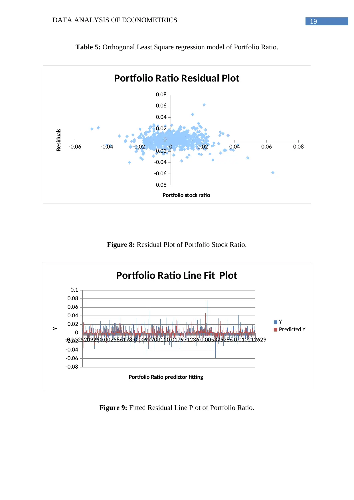
Table 5: Orthogonal Least Square regression model of Portfolio Ratio.
-0.06 -0.04 -0.02 0 0.02 0.04 0.06 0.08
-0.08
-0.06
-0.04
-0.02
0
0.02
0.04
0.06
0.08
Portfolio Ratio Residual Plot
Portfolio stock ratio
Residuals
Figure 8: Residual Plot of Portfolio Stock Ratio.
-0.0025209260.002586178-0.0097703110.017971236 0.005375286 0.010212629
-0.08
-0.06
-0.04
-0.02
0
0.02
0.04
0.06
0.08
0.1
Portfolio Ratio Line Fit Plot
Y
Predicted Y
Portfolio Ratio predictor fitting
Y
Figure 9: Fitted Residual Line Plot of Portfolio Ratio.

DATA ANALYSIS OF ECONOMETRICS 20
0.00 0.02 0.04 0.06 0.08
-1 0 1 2 3 4 5
Leverage
S ta n d a rd iz e d re s id u a ls
lm(sqrt(rp) ~ sqrt(consumer.services.stock) + sqrt(healthcare.stock) + sqrt ...
Cook's distance
0.5
Residuals vs Leverage
5
506232
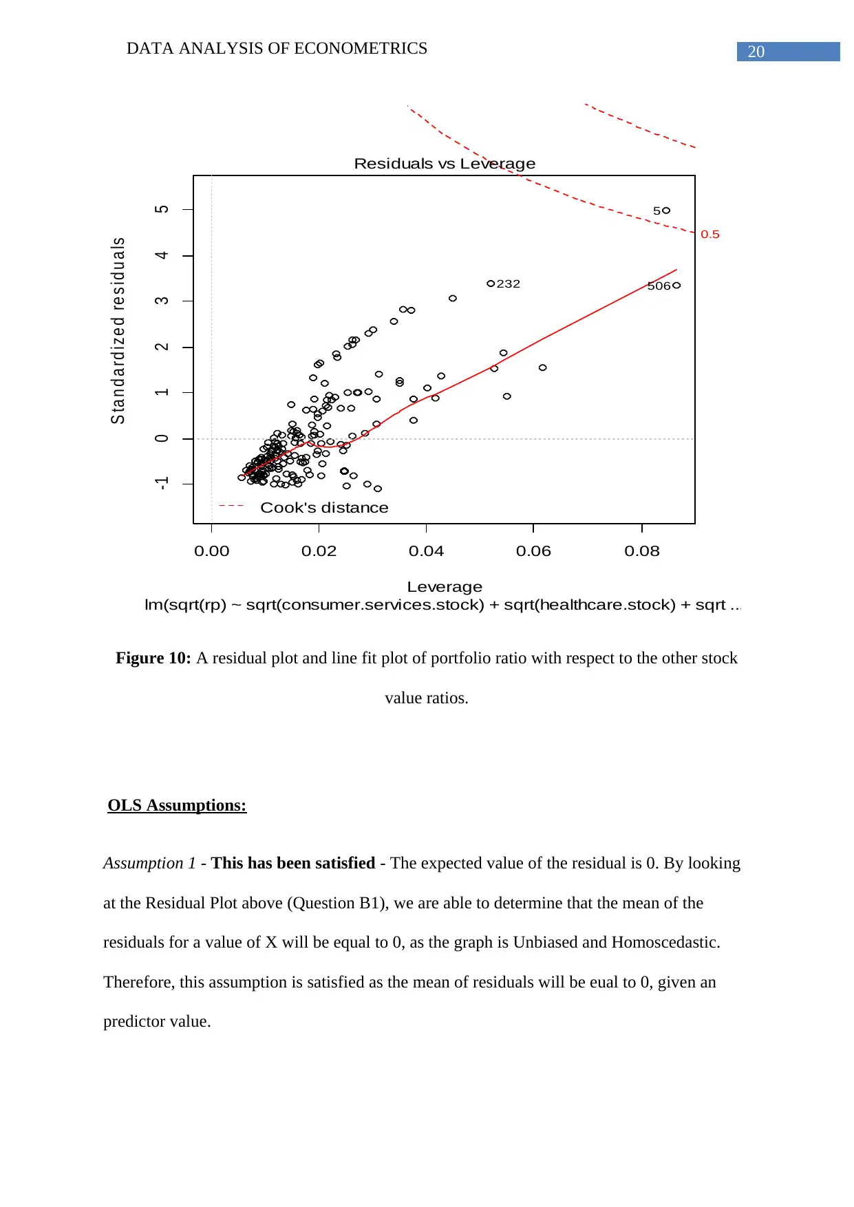
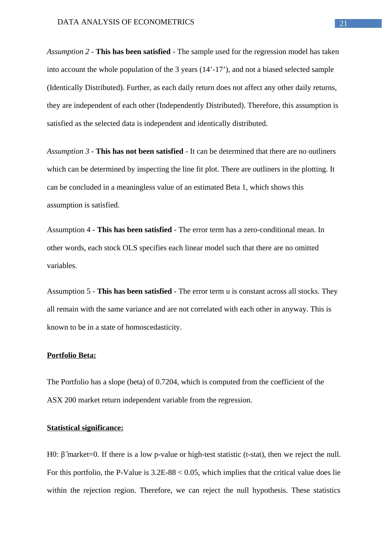
Figure 10: A residual plot and line fit plot of portfolio ratio with respect to the other stock
value ratios.
OLS Assumptions:
Assumption 1 - This has been satisfied - The expected value of the residual is 0. By looking
at the Residual Plot above (Question B1), we are able to determine that the mean of the
residuals for a value of X will be equal to 0, as the graph is Unbiased and Homoscedastic.
Therefore, this assumption is satisfied as the mean of residuals will be eual to 0, given an
predictor value.

DATA ANALYSIS OF ECONOMETRICS 21
Assumption 2 - This has been satisfied - The sample used for the regression model has taken
into account the whole population of the 3 years (14’-17’), and not a biased selected sample
(Identically Distributed). Further, as each daily return does not affect any other daily returns,
they are independent of each other (Independently Distributed). Therefore, this assumption is
satisfied as the selected data is independent and identically distributed.
Assumption 3 - This has not been satisfied - It can be determined that there are no outliners
which can be determined by inspecting the line fit plot. There are outliners in the plotting. It
can be concluded in a meaningless value of an estimated Beta 1, which shows this
assumption is satisfied.
Assumption 4 - This has been satisfied - The error term has a zero-conditional mean. In
other words, each stock OLS specifies each linear model such that there are no omitted
variables.
Assumption 5 - This has been satisfied - The error term u is constant across all stocks. They
all remain with the same variance and are not correlated with each other in anyway. This is
known to be in a state of homoscedasticity.
Portfolio Beta:
The Portfolio has a slope (beta) of 0.7204, which is computed from the coefficient of the
ASX 200 market return independent variable from the regression.
Statistical significance:
H0: β ̂ market=0. If there is a low p-value or high-test statistic (t-stat), then we reject the null.
For this portfolio, the P-Value is 3.2E-88 < 0.05, which implies that the critical value does lie
within the rejection region. Therefore, we can reject the null hypothesis. These statistics

DATA ANALYSIS OF ECONOMETRICS 22
indicate that the market does have a statistically significant impact on the returns of this
portfolio.
This Beta is in line with our expectations for the following reasons:
Stock Beta
Adelaide Brighton 0.0204 (4dp)
WEBJET 0.04761 (4dp)
RAMSAY Healthcare 0.08542 (4dp)
Portfolio (Average) 0.0374758
Thus, the average of portfolio beta is 0.0374758, which is in line with the regression beta of
0.7204 as our expectations.
R2 (Line of best fit)
The Portfolio R2 indicated that 0.63109 or 63.10% of the variance in the portfolio
return is correlated to the market index. This can be justified by the characteristics of the
portfolio relative to each stock in the portfolio’s risk.
Expectations of the Portfolio’s line of best fit
From B4, we have analyzed the R2 for each stock contained within the portfolio and
can be compared to the portfolio’s R2 of 63.10%, we expected that Adelaide Brighton’s
R2 carries more of an impact on the portfolio compared to the other R2 stocks, which the other
R2 stocks offset’s Adelaide Brighton’s R2 resulting to the computed portfolio R2.
Portfolio Diversification

DATA ANALYSIS OF ECONOMETRICS 23
Diversification is an investment strategy which protects an investor for unsystematic
risk, by diversifying is done by investing into a variety of stock from various industries, this
restrict the portfolio to be impacted by unsystematic risk which the risk coming from the
market, this can be quantified by the market beta.
Since the portfolio’s beta is 0.63109, it is safe to conclude that the portfolio is
diversified because its beta is less than 1.The measure of fit for the portfolio comparison with
the measures of fit for our individual stocks shows that portfolio stock is far more nicely
fitted. The portfolio diversification effect using our R2s interprets that all the stock values are
significant to the portfolio stock value.
Question C (Population Survey):
C1.
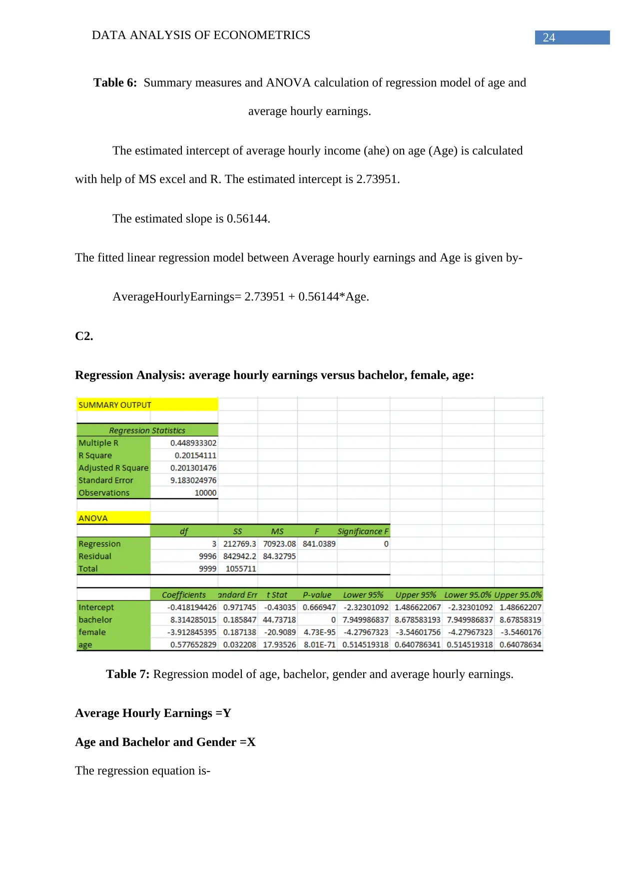
AHE=Y Age=X

DATA ANALYSIS OF ECONOMETRICS 24
Table 6: Summary measures and ANOVA calculation of regression model of age and
average hourly earnings.
The estimated intercept of average hourly income (ahe) on age (Age) is calculated
with help of MS excel and R. The estimated intercept is 2.73951.
The estimated slope is 0.56144.
The fitted linear regression model between Average hourly earnings and Age is given by-
AverageHourlyEarnings= 2.73951 + 0.56144*Age.
C2.
Regression Analysis: average hourly earnings versus bachelor, female, age:
Table 7: Regression model of age, bachelor, gender and average hourly earnings.
Average Hourly Earnings =Y
Age and Bachelor and Gender =X
The regression equation is-

DATA ANALYSIS OF ECONOMETRICS 25
ahe = - 0.418 + 8.31*bachelor - 3.91*female + 0.578*age
S = 9.18302 R-Sq = 20.2% R-Sq (adj) = 20.1%
The estimated effect of age on earning is = 0.578. For every increase in one year of
age , average hourly earnings increase by 0.578.
The 95% Confidence Interval for the coefficient of Age on linear regression is given
by = ((0.578+ 1.96*0.0322076677), (0.578-1.96*0.0322076677)) = (0.6408, 0.5145)
C3.
The linear regressions regarding average hourly earnings and age in C1 and C2
substantively are different from each other in the way that-
Coefficients of intercept of age in C1 and C2 are respectively 0.56144 and 0.57765.
The value of intercept is lesser than C2 in case of C1. This bias occurred due to involvement
of more two factors in C2 linear regression model.
The amount of bias is calculated as-
(0.57765- 0.56144) = 0.01621. Therefore, no significant bias is observed.
C4.
Bob is a 26-year-old male worker with a high school diploma. We have to predict
Bob's earnings using the estimated regression in C2.
ahe = - 0.418 + 8.31*bachelor - 3.91*female + 0.578*age
= -0.418 + 8.31* 0 – 3.91*0 + .578*26
= 14.61

DATA ANALYSIS OF ECONOMETRICS 26
Alexis is a30-year-old female worker with a college degree. We have to predict
Alexis’s earning using the estimated regression in C2.
ahe = - 0.418 + 8.31*bachelor - 3.91*female + 0.578*age
= -0.418 + 8.31 * 1- 3.91*1 + 0.578*30
ahe = 21.322
C5.
R-square is efficient as it explains the proportion in the variance in response (Y),
which is explained by X. Within multiple regression there is a constant increase in the R-
square due to more variables being introduced in the regression. This does not become a good
fitted model. Therefore, due to this the value of R-square shows inefficiency.
The values of R2 and adjusted R2 of the previous two linear models in C1 and C2 are
(0.0243 and 0.02421) and (0.2015 and 0.2013).
The predictor age has significant effect on the response “average hourly earnings” in
case of C1 regression model. Therefore, the model had less value of residual standard error.
Therefore, the values of residual R2 and adjusted R2 is very near to each other.
Similarly, age, gender and bachelorship have significant effect on the response
“average hourly earnings” in case of C2 regression model. Therefore, the model had less
value of residual standard error. The model in C2 has more appropriateness in case of
goodness of fit.
C6.
a) Average hourly earnings versus gender:
Gender (Female):

DATA ANALYSIS OF ECONOMETRICS 27
Here the p-value at 95% confidence interval is given by = 4.72533E-95. It is less than
0.05. The small p-value also shows that the null hypothesis cannot be accepted. Therefore we
reject the null hypothesis of relationship of Gender with the average hourly earnings.
Therefore, gender factor can be deleted from the data.
b) Average hourly earnings versus bachelor:
Here the p-value at 95% confidence interval is given by = 0. It is less than 0.05. The
small p-value also shows that the null hypothesis cannot be accepted. Therefore we reject the
null hypothesis of relationship of bachelor with the average hourly earnings. Therefore,
bachelor factor can be deleted from the data.
c) Average hourly earnings vs (gender and bachelor):
The two factors bachelor and gender do not have linear effect on average hourly
earnings as individual variables.
-0.4181944 + 8.3143(Bachelor) – 3.9128(Female) + 0.5777(Age)
F critical=F2, d.f of F2= (10000 -3 -1)= 9996, F2=2.9957
F actual = [0.2154111 – (0.02430482 / 2)] / [(1 – 0.2154111) / (10000 -3 – 1)] = 1216.923
According to the value of f-actual (1216.923), it is greater than f-critical. Therefore, null
hypothesis is rejected so both female and male can be deleted from regression.
C7.
Condition1:
Therefore, we can conclude that we could delete and ignore these two factors for their null
effect on the variability of “average hourly earnings”. The omitted variable must be a

DATA ANALYSIS OF ECONOMETRICS 28
determinant of the dependent variable. As the education level has an impact on the Average
Hourly Earnings, then the above condition holds.
Condition2:
Secondly, omitted variable must be correlated with an independent variable specified
in the regression. Since, the education level and gender is not correlated with the age, there is
not enough evidence to suggest this condition holds.

DATA ANALYSIS OF ECONOMETRICS 29
Conclusion:
The report concludes in the first part that Sydney is most trendy city of Australia. The
interest amount and principal amount of housing is increasing year by year. In the second
part, we have interpreted that portfolio ratio is one of the most favorable ratio than other
stock ratio. The report also helped us to test various hypotheses and draw necessary
inferences about age and other factors about average hourly earnings in the thirdpart.

DATA ANALYSIS OF ECONOMETRICS 30
Bibliography List:
Cruz, C.D., 2013. Genes: a software package for analysis in experimental statistics and
quantitative genetics. Acta Scientiarum. Agronomy, 35(3), pp.271-276.
Guo, Y., Guo, L.Z., Billings, S.A. and Wei, H.L., 2015. Identification of nonlinear systems
with non-persistent excitation using an iterative forward orthogonal least squares regression
algorithm. International Journal of Modelling, Identification and Control, 23(1), pp.1-7.
Kazem, A., Sharifi, E., Hussain, F.K., Saberi, M. and Hussain, O.K., 2013. Support vector
regression with chaos-based firefly algorithm for stock market price forecasting. Applied soft
computing, 13(2), pp.947-958.
O Schabenberger, CA Gotway – 2017, Statistical methods for spatial data analysis,
books.google.com
P Bazeley, K Jackson – 2013, Qualitative data analysis with NVivo, (450-1)
Pfister, R., Schwarz, K., Carson, R. and Jancyzk, M., 2013. Easy methods for extracting
individual regression slopes: comparing SPSS, R, and Excel. Tutor. Quant. Methods
Psychol, 9(2), pp.72-78.
RL Ott, MT Longnecker - 2015 , An introduction to statistical methods and data analysis,
Nelson Education
Slezák, P., Bokes, P., Námer, P. and Waczulíková, I., 2014. Microsoft Excel add-in for the
statistical analysis of contingency tables. International Journal for Innovation Education and
Research, 2(5), pp.90-100.
Wang, N., Er, M.J. and Han, M., 2014. Parsimonious extreme learning machine using
recursive orthogonal least squares. IEEE transactions on neural networks and learning
systems, 25(10), pp.1828-1841.

DATA ANALYSIS OF ECONOMETRICS 31

DATA ANALYSIS OF ECONOMETRICS 32

DATA ANALYSIS OF ECONOMETRICS 33

DATA ANALYSIS OF ECONOMETRICS 34