Data Analysis for Finance and Economics

This report covers statistical data analysis techniques for finance and economics. It includes correlation, normal distribution, probability, central tendency, quartiles, dispersion, regression analysis, and hypothesis testing.

Data analysis for
finance and economics

Contents
Contents...................................................................................................................................................2
INTRODUCTION...................................................................................................................................3
QUESTION 1...........................................................................................................................................3
a. Draw a scatter diagram to represent the data.............................................................................3
b. From (a) is the relationship roughly linear? What is the direction?..........................................4
a. Calculate the value of the correlation coefficient r....................................................................4
QUESTION 2...........................................................................................................................................5
QUESTION 3...........................................................................................................................................6
QUESTION 4...........................................................................................................................................8
QUESTION 5.........................................................................................................................................10
(b) Calculation of the regression equations:......................................................................................10
3. Least square regression coefficients..............................................................................................10
(c) squared correlation coefficient.....................................................................................................11
d) comment on the regression line.....................................................................................................12
QUESTION 6.........................................................................................................................................12
QUESTION 7.........................................................................................................................................13
QUESTION 8.........................................................................................................................................13
CONCLUSION......................................................................................................................................17
References................................................................................................................................................1

INTRODUCTION
Data can be defined as a set of figures or information that is used to generate information
about the topic. By analyzing this data, an analyst can draw a lot of information that can be used for
taking decision. It helps companies in managing the operations if the company and bringing out
effective results out of it (Ravid, 2019). The report is based on the calculation and analysis of
statistical data with the help of various techniques. There are seven questions under this report. The
first one deals in correlation. The second one prepares a normal distribution and its graph. The third
query is about the probability and forth question prepares central tendency, quartiles and dispersion.
The fifth one calculates the correlation coefficient and regression analysis. The sixth question
conducts the Z – test for the hypothesis. The seventh sections construct a tree diagram and the eighth
one interprets the estimations in regression equation.
QUESTION 1
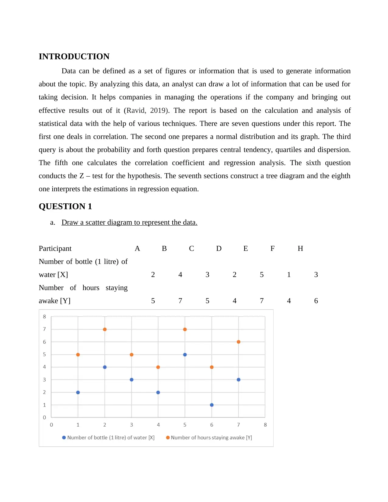
a. Draw a scatter diagram to represent the data.
Participant A B C D E F H
Number of bottle (1 litre) of
water [X] 2 4 3 2 5 1 3
Number of hours staying
awake [Y] 5 7 5 4 7 4 6

b. From (a) is the relationship roughly linear? What is the direction?
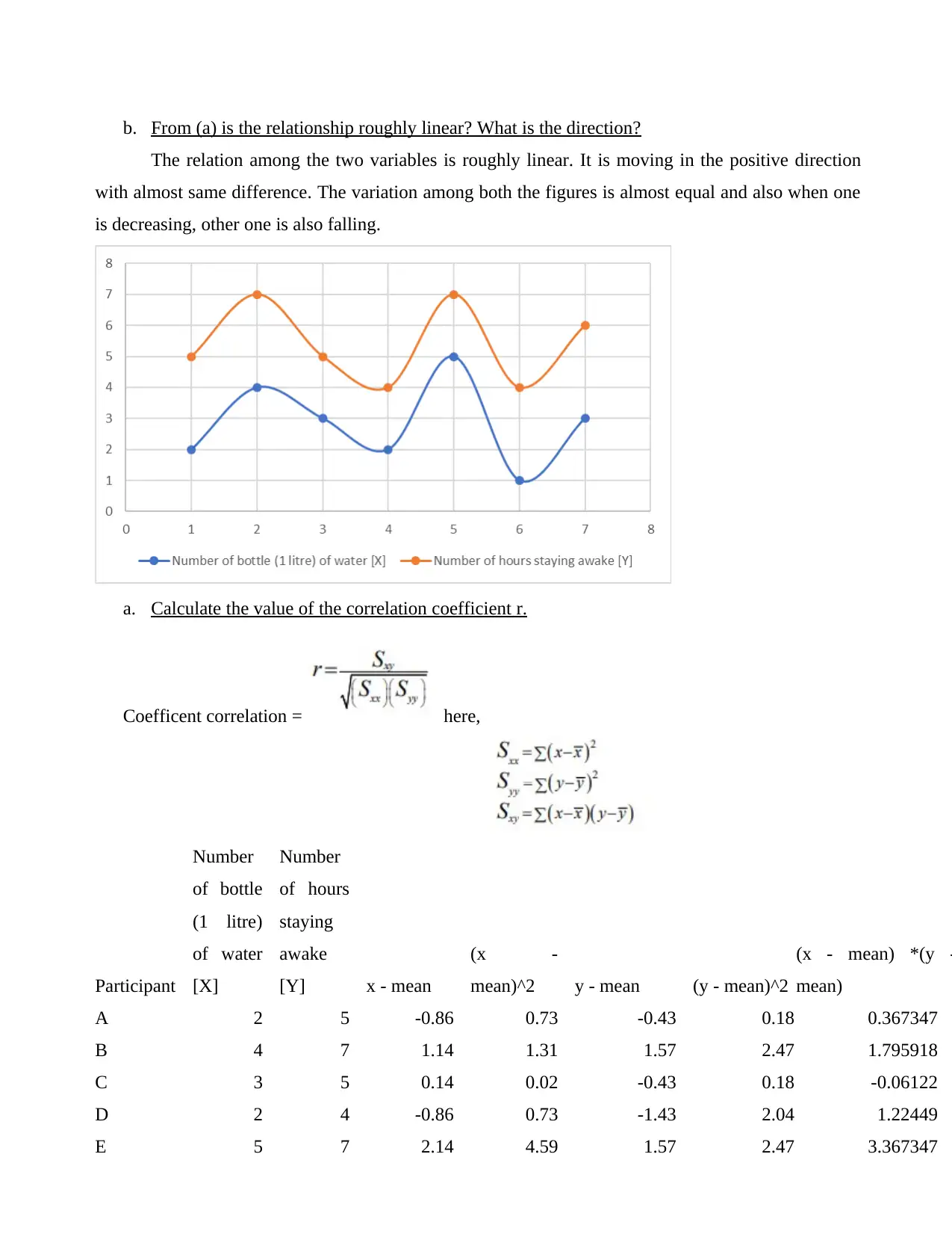
The relation among the two variables is roughly linear. It is moving in the positive direction
with almost same difference. The variation among both the figures is almost equal and also when one
is decreasing, other one is also falling.
a. Calculate the value of the correlation coefficient r.
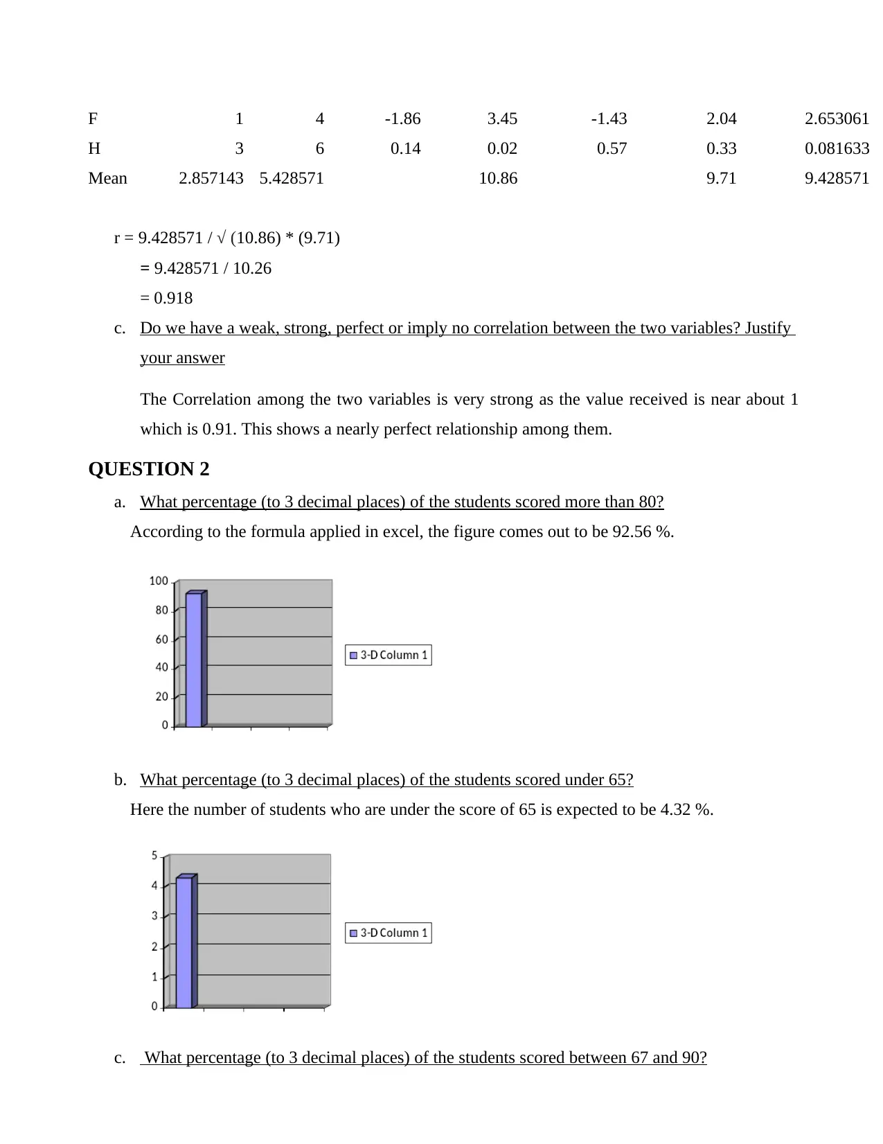
Coefficent correlation = here,
Participant
Number
of bottle
(1 litre)
of water
[X]
Number
of hours
staying
awake
[Y] x - mean
(x -
mean)^2 y - mean (y - mean)^2
(x - mean) *(y -
mean)
A 2 5 -0.86 0.73 -0.43 0.18 0.367347
B 4 7 1.14 1.31 1.57 2.47 1.795918
C 3 5 0.14 0.02 -0.43 0.18 -0.06122
D 2 4 -0.86 0.73 -1.43 2.04 1.22449
E 5 7 2.14 4.59 1.57 2.47 3.367347

F 1 4 -1.86 3.45 -1.43 2.04 2.653061
H 3 6 0.14 0.02 0.57 0.33 0.081633
Mean 2.857143 5.428571 10.86 9.71 9.428571
r = 9.428571 / √ (10.86) * (9.71)
= 9.428571 / 10.26
= 0.918
c. Do we have a weak, strong, perfect or imply no correlation between the two variables? Justify
your answer
The Correlation among the two variables is very strong as the value received is near about 1
which is 0.91. This shows a nearly perfect relationship among them.
QUESTION 2
a. What percentage (to 3 decimal places) of the students scored more than 80?
According to the formula applied in excel, the figure comes out to be 92.56 %.
b. What percentage (to 3 decimal places) of the students scored under 65?
Here the number of students who are under the score of 65 is expected to be 4.32 %.
c. What percentage (to 3 decimal places) of the students scored between 67 and 90?

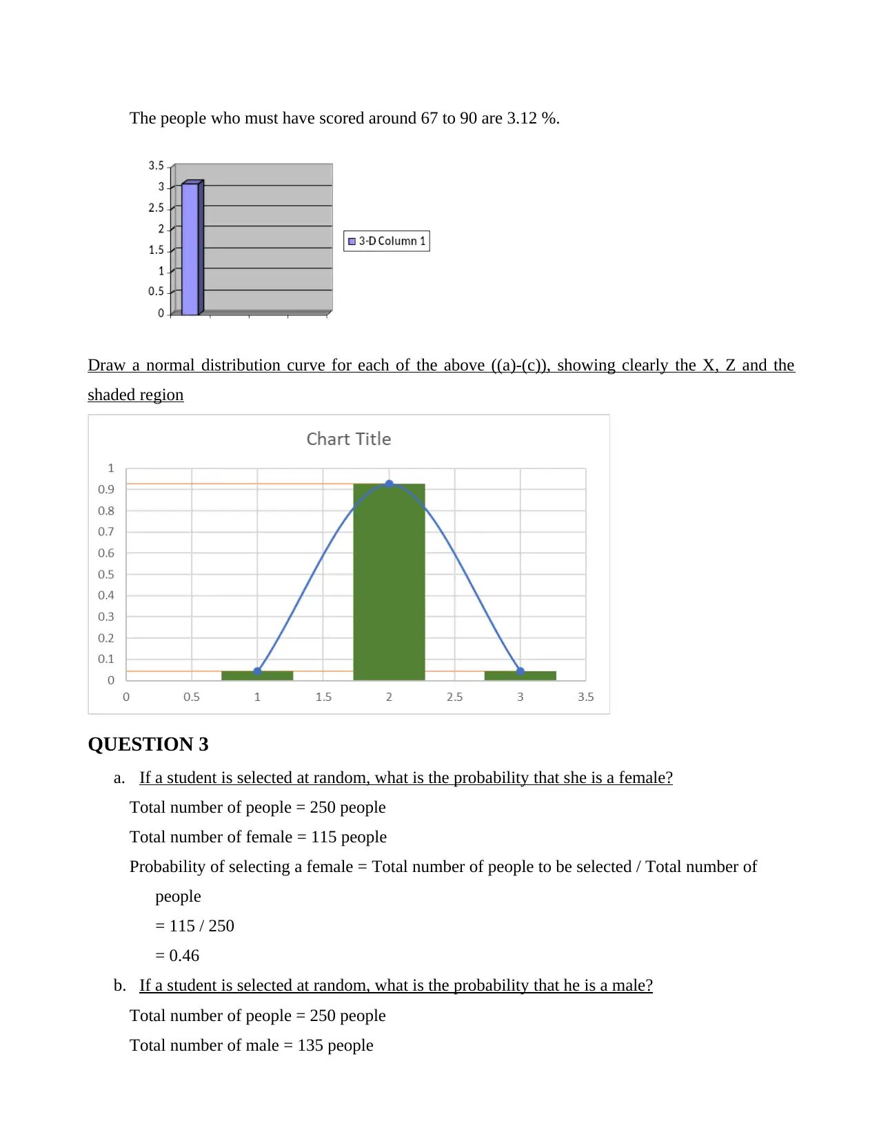
The people who must have scored around 67 to 90 are 3.12 %.
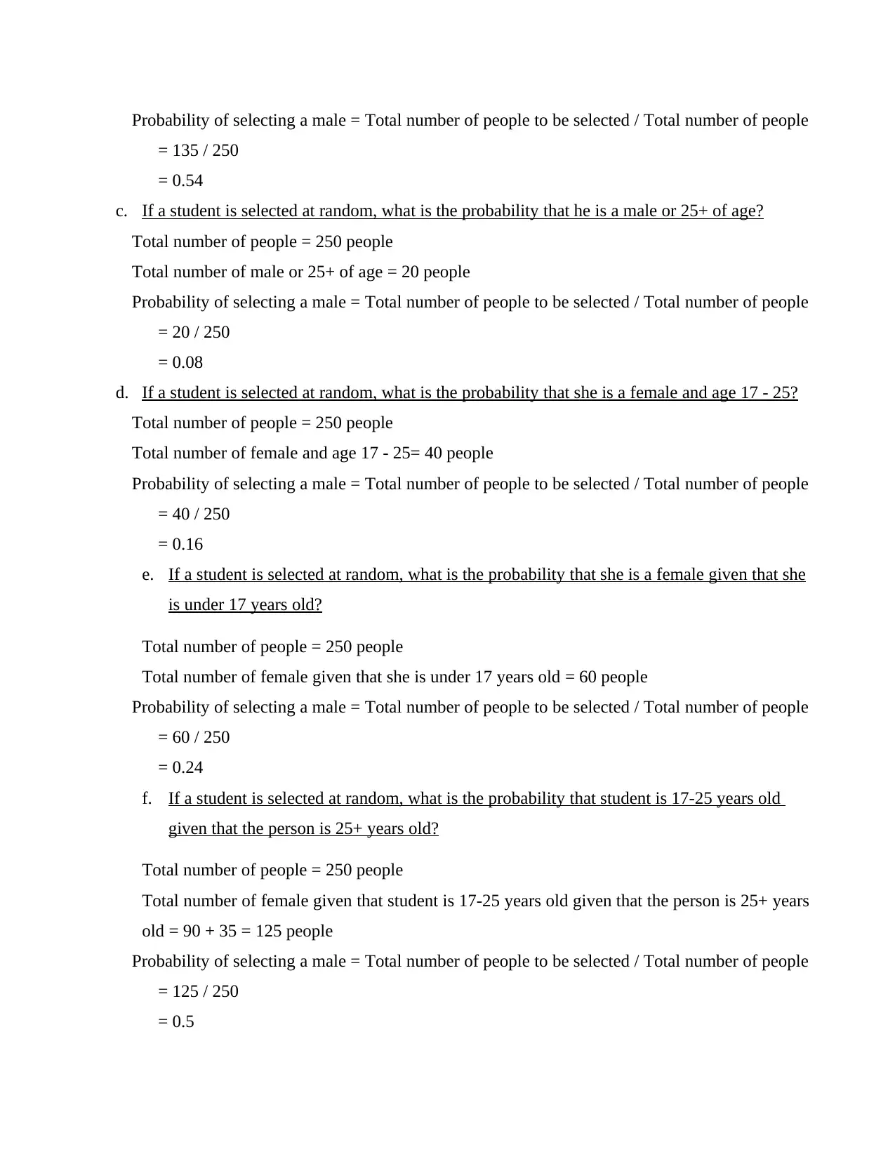
Draw a normal distribution curve for each of the above ((a)-(c)), showing clearly the X, Z and the
shaded region
QUESTION 3
a. If a student is selected at random, what is the probability that she is a female?
Total number of people = 250 people
Total number of female = 115 people
Probability of selecting a female = Total number of people to be selected / Total number of
people
= 115 / 250
= 0.46
b. If a student is selected at random, what is the probability that he is a male?
Total number of people = 250 people
Total number of male = 135 people

Probability of selecting a male = Total number of people to be selected / Total number of people
= 135 / 250
= 0.54
c. If a student is selected at random, what is the probability that he is a male or 25+ of age?
Total number of people = 250 people
Total number of male or 25+ of age = 20 people
Probability of selecting a male = Total number of people to be selected / Total number of people
= 20 / 250
= 0.08
d. If a student is selected at random, what is the probability that she is a female and age 17 - 25?
Total number of people = 250 people
Total number of female and age 17 - 25= 40 people
Probability of selecting a male = Total number of people to be selected / Total number of people
= 40 / 250
= 0.16
e. If a student is selected at random, what is the probability that she is a female given that she
is under 17 years old?
Total number of people = 250 people
Total number of female given that she is under 17 years old = 60 people
Probability of selecting a male = Total number of people to be selected / Total number of people
= 60 / 250
= 0.24
f. If a student is selected at random, what is the probability that student is 17-25 years old
given that the person is 25+ years old?
Total number of people = 250 people
Total number of female given that student is 17-25 years old given that the person is 25+ years
old = 90 + 35 = 125 people
Probability of selecting a male = Total number of people to be selected / Total number of people
= 125 / 250
= 0.5

QUESTION 4
a. Mode and Median
Mode is 12 as this test score is having the maximum frequency of 9. The higher occurring
frequency is always termed as mode which in this case is 12.
Median is the central figure of the table after sorting the intervals in ascending order.
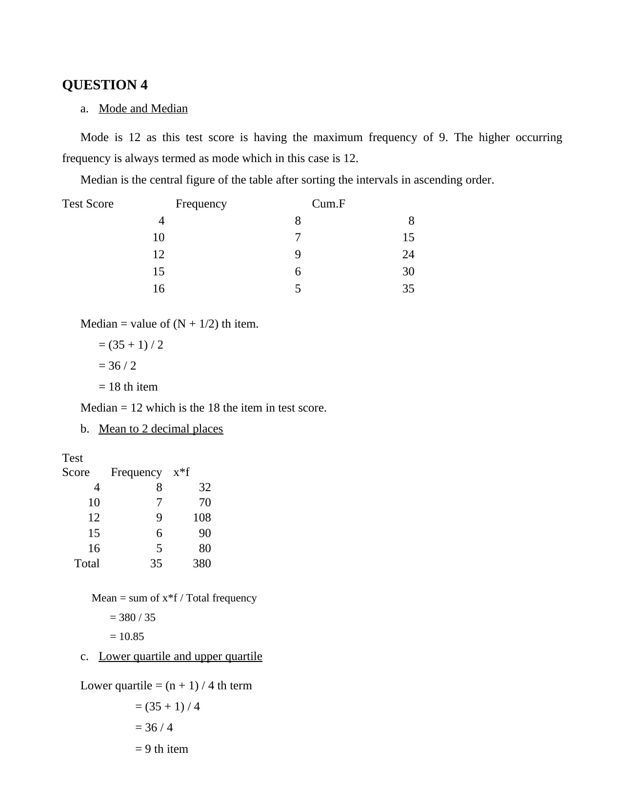
Test Score Frequency Cum.F
4 8 8
10 7 15
12 9 24
15 6 30
16 5 35
Median = value of (N + 1/2) th item.
= (35 + 1) / 2
= 36 / 2
= 18 th item
Median = 12 which is the 18 the item in test score.
b. Mean to 2 decimal places
Test
Score Frequency x*f
4 8 32
10 7 70
12 9 108
15 6 90
16 5 80
Total 35 380
Mean = sum of x*f / Total frequency
= 380 / 35
= 10.85
c. Lower quartile and upper quartile
Lower quartile = (n + 1) / 4 th term
= (35 + 1) / 4
= 36 / 4
= 9 th item

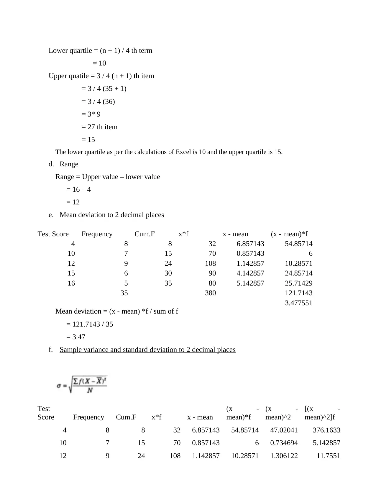
Lower quartile = (n + 1) / 4 th term
= 10
Upper quatile = 3 / 4 (n + 1) th item
= 3 / 4 (35 + 1)
= 3 / 4 (36)
= 3* 9
= 27 th item
= 15
The lower quartile as per the calculations of Excel is 10 and the upper quartile is 15.
d. Range
Range = Upper value – lower value
= 16 – 4
= 12
e. Mean deviation to 2 decimal places
Test Score Frequency Cum.F x*f x - mean (x - mean)*f
4 8 8 32 6.857143 54.85714
10 7 15 70 0.857143 6
12 9 24 108 1.142857 10.28571
15 6 30 90 4.142857 24.85714
16 5 35 80 5.142857 25.71429
35 380 121.7143
3.477551
Mean deviation = (x - mean) *f / sum of f
= 121.7143 / 35
= 3.47
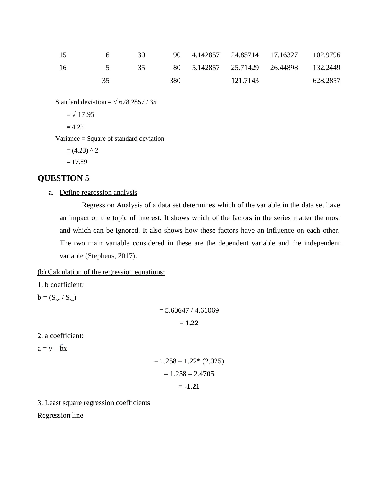
f. Sample variance and standard deviation to 2 decimal places
Test
Score Frequency Cum.F x*f x - mean
(x -
mean)*f
(x -
mean)^2
[(x -
mean)^2]f
4 8 8 32 6.857143 54.85714 47.02041 376.1633
10 7 15 70 0.857143 6 0.734694 5.142857
12 9 24 108 1.142857 10.28571 1.306122 11.7551

15 6 30 90 4.142857 24.85714 17.16327 102.9796
16 5 35 80 5.142857 25.71429 26.44898 132.2449
35 380 121.7143 628.2857
Standard deviation = √ 628.2857 / 35
= √ 17.95
= 4.23
Variance = Square of standard deviation
= (4.23) ^ 2
= 17.89
QUESTION 5
a. Define regression analysis
Regression Analysis of a data set determines which of the variable in the data set have
an impact on the topic of interest. It shows which of the factors in the series matter the most
and which can be ignored. It also shows how these factors have an influence on each other.
The two main variable considered in these are the dependent variable and the independent
variable (Stephens, 2017).
(b) Calculation of the regression equations:
1. b coefficient:
b = (Sxy / Sxx)
= 5.60647 / 4.61069
= 1.22
2. a coefficient:
a = y – bx
= 1.258 – 1.22* (2.025)
= 1.258 – 2.4705
= -1.21
3. Least square regression coefficients
Regression line

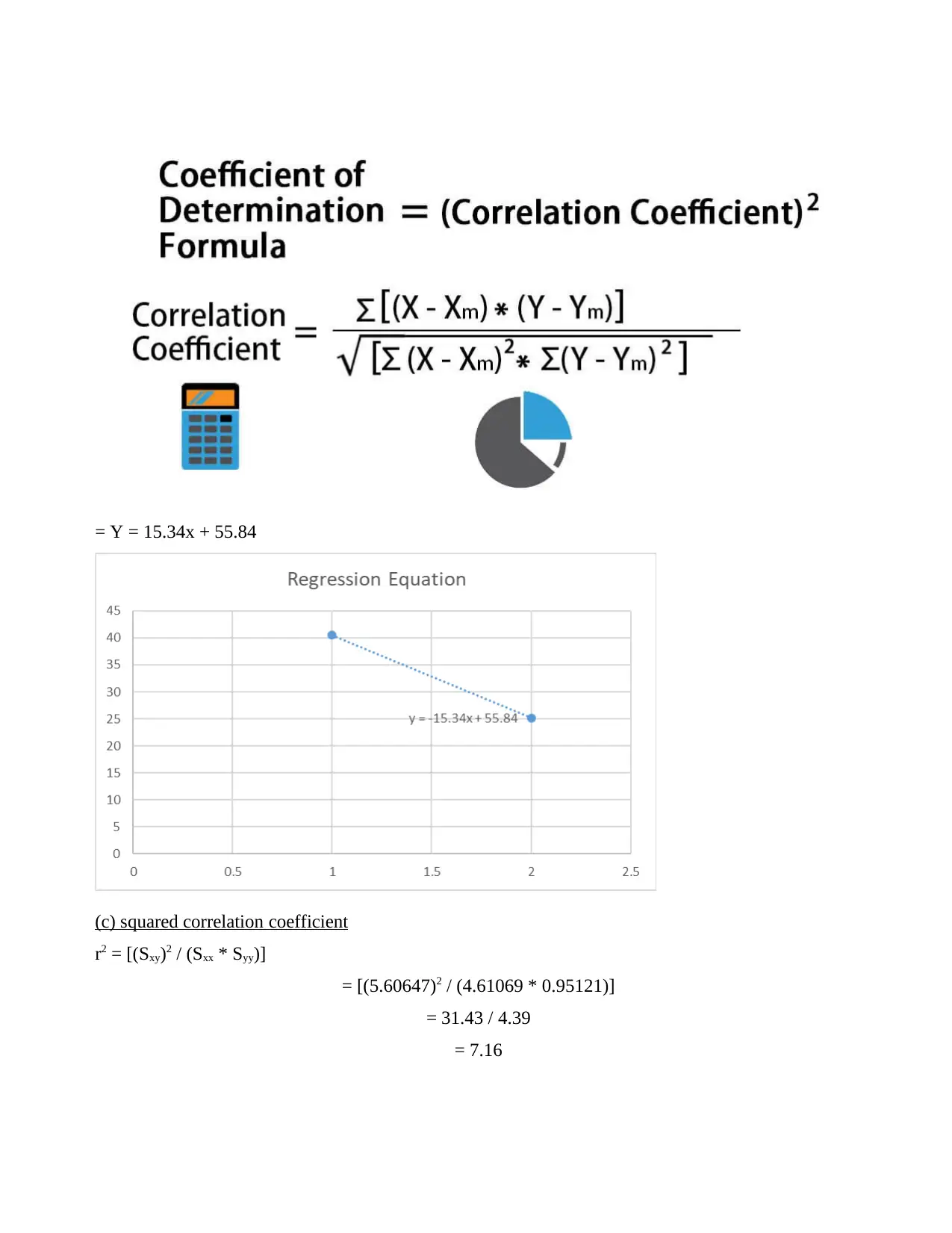
= Y = 15.34x + 55.84
(c) squared correlation coefficient
r2 = [(Sxy)2 / (Sxx * Syy)]
= [(5.60647)2 / (4.61069 * 0.95121)]
= 31.43 / 4.39
= 7.16

d) comment on the regression line.
The above mentioned regression line is not s good fit as the value of correlation is nor between 1
and -1. The line which has more errors of sum of squares is treated to be bad an dthe above line is
very much diversified.
QUESTION 6
Ho: p = 6.25
Ha: p ≠ 6.25
critical value = 1.96
z test statistic = -2.874
p value = 0.0041
Decision = Reject the null hypothesis
Conclusion = There is enough evidence to reject the claim.
Z Test for One Population Proportion
Null and Alternative hypotheses
Null hypothesis Ho: p = 0.87
Alternative hypothesis Ha: p ≠ 0.87
This is a two-tailed test
Rejection Region
level of significance = 0.05. Using z distribution, the critical value is 1.96
Critical value approach = Reject Ho if z > critical value, or Reject Ho if z > 1.96
P value approach: Reject Ho if p < significance level, or Reject Ho if p < 0.05
Test Statistic
Given
x = 371
n = 450
Sample proportion p̂ = 371/450 = 0.8244
Hypothesized proportion po = 0.87
Solution
z = -2.874
Decision on Ho
Critical value approach: Since z . zc or 2.874 > 1.96, then the null hypothesis is rejected.
Probability for the z score of -2.874 is 0.0041

Using Microsoft excel, the two-tailed p value is
=2*NORM.S.DIST(z score,TRUE)
=2*NORM.S.DIST(-2.874,TRUE)
= 0.0041
Therefore, the p value is 0.0041
P value approach: Since p < alpha or 0.0041 < 0.05, then the Null hypothesis is Rejected.
QUESTION 7
a. How many sample points are there for this experiment? List the sample points.
In step 1 there is 1 positive and 1 negative alternative
In step 2 there is 1 positive and 1 negative alternative
So there is 2*2=4 sample points.
b. Construct a tree diagram for the experiment.
QUESTION 8
1. In a regression analysis involving 30 observations, the following estimated regression
equation was obtained

ŷ = 17.6 + 3.8x1 – 2.3x2 + 7.6x3 + 2.7x4
and thus interpreted as:
b1= 3.8 is the estimate expected value when x2, x3, and x4 are held constant; b2= -2.3 is the estimate
expected value when x1, x3, and x4 are held constant; b3= 7.6 is the estimate expected value when x1, x2,
and x4 are held constant and; b4= 2.7 is the estimate expected value when x1, x2, and x3 are held
constant.
a. The prediction of the value of ŷ when x1=20, x2=30, x3=5 and x4=2 is 10.
2. a. The estimated regression equation relating y to x1 is y = 1.9436x1 + 45.059.
The prediction of the value of ŷ when x1=45 is 132.521.
Regression Statistics
Multiple R 0.778693888
Relationship of y to x1
y Linear (y)
250
200 f(x) = 1.94 x + 45.06
R² = 0.66
150
100
50
0
20 30 40 50 60 70 80
X1

Relationship of y to x2
y Linear (y)
250
200
150
100
50
04 6 8 10 12
X2
14 16 18 20
R Square 0.606364172
Adjusted R Square 0.550130482
Standard Error 26.85150605
Observations 9
df SS MS F Significance
Upper
Lower 99.0% Upper
95% 99.0%
121.93229 -55.0991511 156.192531
7
3.193167 -0.12196656 3.83473252
1
f(x) =4.32 x + 85.22
R² = 0.22
F
Regression 1 7774.531915 7774.531915 10.78293412 0.013417768
Residual 7 5047.023641 721.0033772
Total 8 12821.55556
Coefficients Standard Error t Stat P-value Lower 95%
Intercept 50.54669031 30.1889829 1.674342275 0.137975207 -20.83891079
x1 1.856382979 0.565326185 3.283737827 0.013417768 0.519598971

b. The estimated regression equation relating y to x2 is y = 4.3215x2 + 85.217. The
prediction of the value of ŷ when x2=15 is 150.0395.
Regression Statistics
Multiple R 0.489321366
R Square 0.239435399
Adjusted R Square 0.130783313
Standard Error 37.32410421
Observations 9
df SS MS F Significance
95% 99.0% 99.0%
181.54145 -39.5545949 224.329347
4
10.721362 -5.61261362 13.8824156
CONCLUSION
The statistics is an essential concept for an analyst. It helps it in interpreting the figures and deriving
out some useful results out of it. There are various tools that helps them in evaluating the data and
bringing out the essence of that content.
y
F
Regression 1 3069.934268 3069.934268 2.20368893 0.181256643
Residual 7 9751.621287 1393.088755
Total 8 12821.55556
Coefficients Standard Error t Stat P-value Lower 95%
Intercept 92.38737624 37.70327215 2.450380854 0.044082638 3.233304538
x2 4.13490099 2.785415384 1.484482715 0.181256643 -2.451559777
Upper Lower Upper

References
Dietrich, C.F., 2017. Uncertainty, Calibration and Probability: The Adam Hilger Series on
Measurement Science and Technology: The Statistics of Scientific and Industrial
Measurement. Routledge.
Florens, J.P., Mouchart, M. and Rolin, J.M., 2019. Elements of Bayesian statistics. CRC Press.
Kemsley, E.K., Defernez, M. and Marini, F., 2019. Multivariate statistics: Considerations and
confidences in food authenticity problems. Food Control. 105. pp.102-112.
Parzen, E., 2020. Concrete statistics. In Statistics of quality (pp. 309-332). CRC Press.
Ravid, R., 2019. Practical statistics for educators. Rowman & Littlefield Publishers.
Sall, J., Stephens, M.L., Lehman, A. and Loring, S., 2017. JMP start statistics: a guide to
statistics and data analysis using JMP. Sas Institute.
Stephens, M.A., 2017. Tests based on EDF statistics. In Goodness-of-fit Techniques (pp. 97-
194). Routledge..