Data Analysis of Population Estimates for Railway Station Passengers
VerifiedAdded on 2020/05/11
|11
|2113
|194
Report
AI Summary
This report presents a comprehensive data analysis of population estimates based on a survey of passengers accessing railway stations in various Australian cities. The study, conducted for Transport for Victoria, analyzes data collected through a questionnaire-based survey, focusing on factors related to travel from home to the railway station. The analysis includes data cleaning, response rate assessment, and graphical estimations of survey variables. Population estimates are calculated using the Orthogonal Least Square (OLS) method of linear regression, with separate analyses for male, female, and total passengers. The report provides regression equations, R-squared values, and p-values to assess the relationships between passenger numbers and postcard deliveries. Findings reveal insights into passenger demographics, trip purposes, and transportation preferences, concluding with recommendations to improve bicycle usage and address issues at less popular stations. The report uses MINITAB and MS Excel for data processing and presentation.

Running head: DATA ANALYSIS ON POPULATION ESTIMATES
Data Analysis of Population Estimates
Name of the Student:
Name of the University:
Author’s Note:
Data Analysis of Population Estimates
Name of the Student:
Name of the University:
Author’s Note:
Paraphrase This Document
Need a fresh take? Get an instant paraphrase of this document with our AI Paraphraser

DATA ANALYSIS ON POPULATION ESTIMATES 1
Executive Summary:
The following report describes about various factors and aspects of transportation scenario. The data is collected by question-answer set survey
method on different ways to travel from home to railway station Data analysis, testing of hypothesis and data conclusion is elaborately discussed
in the report. Necessary tables and charts were provided in the report; these were calculated with the help of MINITAB and MSexcel. The
necessary measures that could be taken to make bicycle riding more popular are discussed in conclusion part. Railway stations are analyzed
according to the total passengers and total postcards delivered. The population estimation with the help of Orthogonal Least Square (OLS) and
graphs for different railway stations are calculated and measured.

DATA ANALYSIS ON POPULATION ESTIMATES 2
Table of Contents
Introduction and Background:-....................................................................................................................................................................................3
Data Collection:-..........................................................................................................................................................................................................3
Data Description:-........................................................................................................................................................................................................3
Data Analysis and Discussion of each finding:-..........................................................................................................................................................3
Survey Response Rate:-............................................................................................................................................................................................3
Graphical estimation of survey variables:-...............................................................................................................................................................4
Population Estimation (By OLS Method of Linear Regression):-...............................................................................................................................4
Conclusion:-.................................................................................................................................................................................................................9
References:-................................................................................................................................................................................................................10
⊘ This is a preview!⊘
Do you want full access?
Subscribe today to unlock all pages.
Trusted by 1+ million students worldwide

DATA ANALYSIS ON POPULATION ESTIMATES 3
Introduction and Background:-
A survey was recently undertaken of passengers accessing railway stations of different cities of Australia. The data is accessible online in
“Moodle” website. We are working for a consulting firm engaged by Transport for Victoria to analyze the results of the survey (Mah and Mitra
2015). After proper analysis with the help of MINITAB, we are preparing a report for transport of Victoria.
The report elaborates about factors and their effects of analyzed dataset. The dataset is related to different aspects of travelling from
home to railway station. The data is collected by survey method of questionnaire set (Salaria 2012).
Status of Railway stations are also analyzed according to the total passengers and total postcards delivered.
Data Collection:-
A questionnaire set of multiple questions were formed for the collection of the data and their responses were taken as the datasets. Some
of them are numerical in nature and some of them are categorical. The dataset is full of missing values. Firstly the task of data analysis is data
cleaning. We eliminate those factors that have lots of missing values. Secondly, we delete the rows that still have more than 4 missing values.
The big data now becomes less erroneous and composed; such that no difficulty would grow to handle the dataset. The survey data is analyzed to
indicate the estimation of different station (Kahneman 2004).
Data Description:-
The dataset have total nine factors each having more than 500 samples. Distance from station in km, time elapsed to reach station from
home and range of age limit are numeric in nature. Therefore they have scale parameter. The all other variables are categorical in nature.
Data Analysis and Discussion of each finding:-
Survey Response Rate:-
At which railway station were you handed the postcard for this survey? 614 responses
Is this the station where you regularly catch the train? 614 responses
If not, which station do you regularly catch the train? 28 responses
What is your trip purpose? 632 responses
In a typical week, how often do you travel by train? 632 responses
What is the distance to station (km) from your home? 614 responses
What is the travel time to station (by car - minutes)? 614 responses
How do you usually get to the train station from home? 632 responses
What gender do you associate with? 632 responses
What is your age range? 632 responses
The major function of this research is found to be well researched. Out of 634 variables, most of the variables responded positively over 90%
questions. Therefore, we can say that response rate of questions among answerers is very high.
Paraphrase This Document
Need a fresh take? Get an instant paraphrase of this document with our AI Paraphraser
DATA ANALYSIS ON POPULATION ESTIMATES 4
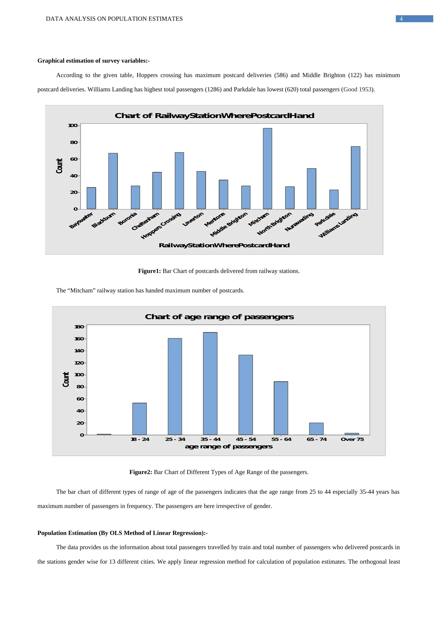
Graphical estimation of survey variables:-
According to the given table, Hoppers crossing has maximum postcard deliveries (586) and Middle Brighton (122) has minimum
postcard deliveries. Williams Landing has highest total passengers (1286) and Parkdale has lowest (620) total passengers (Good 1953).
100
80
60
40
20
0
RailwayStationWherePostcardHand
Count
Chart of RailwayStationWherePostcardHand
Figure1: Bar Chart of postcards delivered from railway stations.
The “Mitcham” railway station has handed maximum number of postcards.
Over 7565 - 7455 - 6445 - 5435 - 4425 - 3418 - 24
180
160
140
120
100
80
60
40
20
0
age range of passengers
Count
Chart of age range of passengers
Figure2: Bar Chart of Different Types of Age Range of the passengers.
The bar chart of different types of range of age of the passengers indicates that the age range from 25 to 44 especially 35-44 years has
maximum number of passengers in frequency. The passengers are here irrespective of gender.
Population Estimation (By OLS Method of Linear Regression):-
The data provides us the information about total passengers travelled by train and total number of passengers who delivered postcards in
the stations gender wise for 13 different cities. We apply linear regression method for calculation of population estimates. The orthogonal least
DATA ANALYSIS ON POPULATION ESTIMATES 5
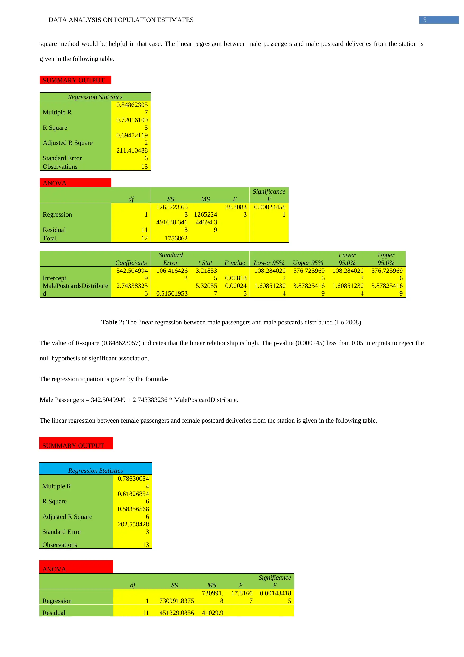
square method would be helpful in that case. The linear regression between male passengers and male postcard deliveries from the station is
given in the following table.
SUMMARY OUTPUT
Regression Statistics
Multiple R
0.84862305
7
R Square
0.72016109
3
Adjusted R Square
0.69472119
2
Standard Error
211.410488
6
Observations 13
ANOVA
df SS MS F
Significance
F
Regression 1
1265223.65
8 1265224
28.3083
3
0.00024458
1
Residual 11
491638.341
8
44694.3
9
Total 12 1756862
Coefficients
Standard
Error t Stat P-value Lower 95% Upper 95%
Lower
95.0%
Upper
95.0%
Intercept
342.504994
9
106.416426
2
3.21853
5 0.00818
108.284020
2
576.725969
6
108.284020
2
576.725969
6
MalePostcardsDistribute
d
2.74338323
6 0.51561953
5.32055
7
0.00024
5
1.60851230
4
3.87825416
9
1.60851230
4
3.87825416
9
Table 2: The linear regression between male passengers and male postcards distributed (Lo 2008).
The value of R-square (0.848623057) indicates that the linear relationship is high. The p-value (0.000245) less than 0.05 interprets to reject the
null hypothesis of significant association.
The regression equation is given by the formula-
Male Passengers = 342.5049949 + 2.743383236 * MalePostcardDistribute.
The linear regression between female passengers and female postcard deliveries from the station is given in the following table.
SUMMARY OUTPUT
Regression Statistics
Multiple R
0.78630054
4
R Square
0.61826854
6
Adjusted R Square
0.58356568
6
Standard Error
202.558428
3
Observations 13
ANOVA
df SS MS F
Significance
F
Regression 1 730991.8375
730991.
8
17.8160
7
0.00143418
5
Residual 11 451329.0856 41029.9
⊘ This is a preview!⊘
Do you want full access?
Subscribe today to unlock all pages.
Trusted by 1+ million students worldwide
DATA ANALYSIS ON POPULATION ESTIMATES 6
2
Total 12 1182320.923
Coefficients
Standard
Error t Stat P-value Lower 95%
Upper
95%
Lower
95.0%
Upper
95.0%
Intercept
228.490614
5 121.2607916
1.88429
1 0.08621
-
38.4025882
495.38381
7
-
38.4025881
7
495.383817
1
FemalePostcardDistribut
ed
3.57154573
7 0.846155674
4.22090
9
0.00143
4
1.70916965
7
5.4339218
2
1.70916965
7
5.43392181
6
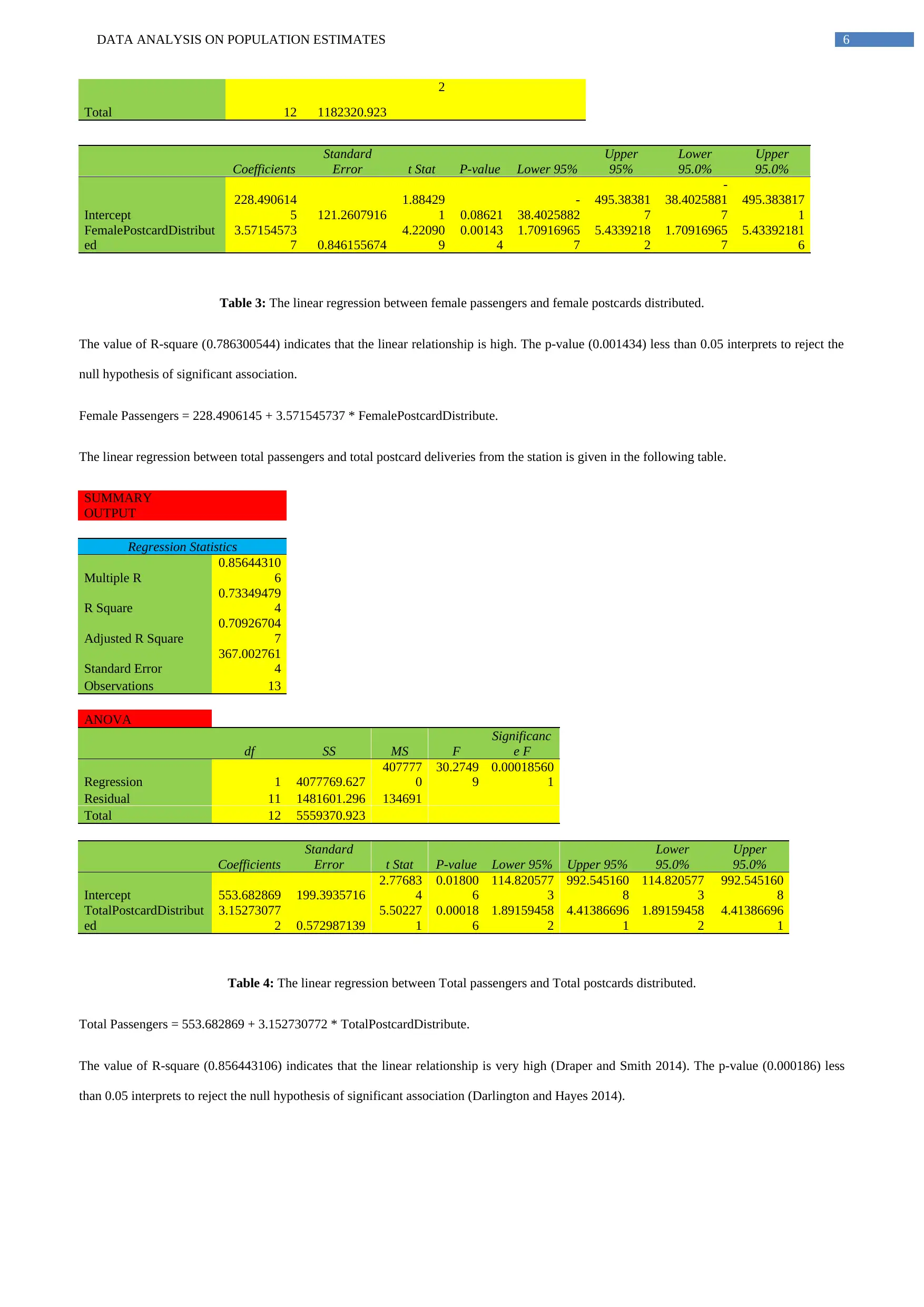
Table 3: The linear regression between female passengers and female postcards distributed.
The value of R-square (0.786300544) indicates that the linear relationship is high. The p-value (0.001434) less than 0.05 interprets to reject the
null hypothesis of significant association.
Female Passengers = 228.4906145 + 3.571545737 * FemalePostcardDistribute.
The linear regression between total passengers and total postcard deliveries from the station is given in the following table.
SUMMARY
OUTPUT
Regression Statistics
Multiple R
0.85644310
6
R Square
0.73349479
4
Adjusted R Square
0.70926704
7
Standard Error
367.002761
4
Observations 13
ANOVA
df SS MS F
Significanc
e F
Regression 1 4077769.627
407777
0
30.2749
9
0.00018560
1
Residual 11 1481601.296 134691
Total 12 5559370.923
Coefficients
Standard
Error t Stat P-value Lower 95% Upper 95%
Lower
95.0%
Upper
95.0%
Intercept 553.682869 199.3935716
2.77683
4
0.01800
6
114.820577
3
992.545160
8
114.820577
3
992.545160
8
TotalPostcardDistribut
ed
3.15273077
2 0.572987139
5.50227
1
0.00018
6
1.89159458
2
4.41386696
1
1.89159458
2
4.41386696
1
Table 4: The linear regression between Total passengers and Total postcards distributed.
Total Passengers = 553.682869 + 3.152730772 * TotalPostcardDistribute.
The value of R-square (0.856443106) indicates that the linear relationship is very high (Draper and Smith 2014). The p-value (0.000186) less
than 0.05 interprets to reject the null hypothesis of significant association (Darlington and Hayes 2014).
2
Total 12 1182320.923
Coefficients
Standard
Error t Stat P-value Lower 95%
Upper
95%
Lower
95.0%
Upper
95.0%
Intercept
228.490614
5 121.2607916
1.88429
1 0.08621
-
38.4025882
495.38381
7
-
38.4025881
7
495.383817
1
FemalePostcardDistribut
ed
3.57154573
7 0.846155674
4.22090
9
0.00143
4
1.70916965
7
5.4339218
2
1.70916965
7
5.43392181
6
Table 3: The linear regression between female passengers and female postcards distributed.
The value of R-square (0.786300544) indicates that the linear relationship is high. The p-value (0.001434) less than 0.05 interprets to reject the
null hypothesis of significant association.
Female Passengers = 228.4906145 + 3.571545737 * FemalePostcardDistribute.
The linear regression between total passengers and total postcard deliveries from the station is given in the following table.
SUMMARY
OUTPUT
Regression Statistics
Multiple R
0.85644310
6
R Square
0.73349479
4
Adjusted R Square
0.70926704
7
Standard Error
367.002761
4
Observations 13
ANOVA
df SS MS F
Significanc
e F
Regression 1 4077769.627
407777
0
30.2749
9
0.00018560
1
Residual 11 1481601.296 134691
Total 12 5559370.923
Coefficients
Standard
Error t Stat P-value Lower 95% Upper 95%
Lower
95.0%
Upper
95.0%
Intercept 553.682869 199.3935716
2.77683
4
0.01800
6
114.820577
3
992.545160
8
114.820577
3
992.545160
8
TotalPostcardDistribut
ed
3.15273077
2 0.572987139
5.50227
1
0.00018
6
1.89159458
2
4.41386696
1
1.89159458
2
4.41386696
1
Table 4: The linear regression between Total passengers and Total postcards distributed.
Total Passengers = 553.682869 + 3.152730772 * TotalPostcardDistribute.
The value of R-square (0.856443106) indicates that the linear relationship is very high (Draper and Smith 2014). The p-value (0.000186) less
than 0.05 interprets to reject the null hypothesis of significant association (Darlington and Hayes 2014).
Paraphrase This Document
Need a fresh take? Get an instant paraphrase of this document with our AI Paraphraser
DATA ANALYSIS ON POPULATION ESTIMATES 7
1 2 3 4 5 6 7 8 9 10 11 12 13
0
200
400
600
800
1000
1200
1400
1600
1800
MalePassengers
EstimatedMalePassengers
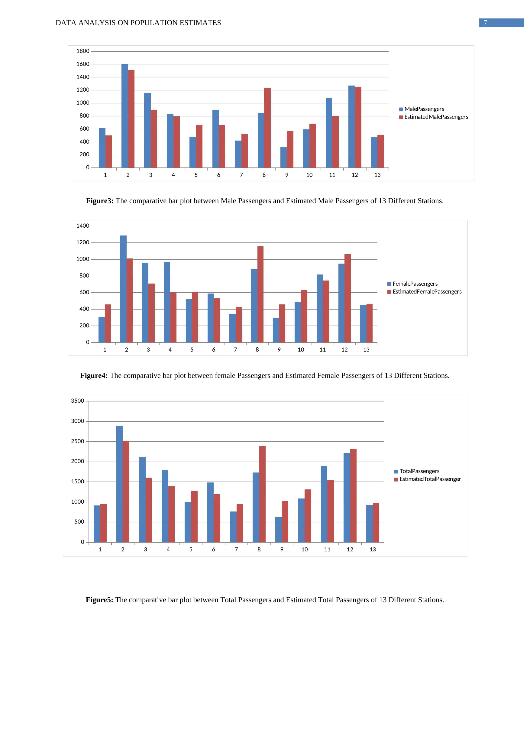
Figure3: The comparative bar plot between Male Passengers and Estimated Male Passengers of 13 Different Stations.
1 2 3 4 5 6 7 8 9 10 11 12 13
0
200
400
600
800
1000
1200
1400
FemalePassengers
EstimatedFemalePassengers
Figure4: The comparative bar plot between female Passengers and Estimated Female Passengers of 13 Different Stations.
1 2 3 4 5 6 7 8 9 10 11 12 13
0
500
1000
1500
2000
2500
3000
3500
TotalPassengers
EstimatedTotalPassenger
Figure5: The comparative bar plot between Total Passengers and Estimated Total Passengers of 13 Different Stations.
1 2 3 4 5 6 7 8 9 10 11 12 13
0
200
400
600
800
1000
1200
1400
1600
1800
MalePassengers
EstimatedMalePassengers
Figure3: The comparative bar plot between Male Passengers and Estimated Male Passengers of 13 Different Stations.
1 2 3 4 5 6 7 8 9 10 11 12 13
0
200
400
600
800
1000
1200
1400
FemalePassengers
EstimatedFemalePassengers
Figure4: The comparative bar plot between female Passengers and Estimated Female Passengers of 13 Different Stations.
1 2 3 4 5 6 7 8 9 10 11 12 13
0
500
1000
1500
2000
2500
3000
3500
TotalPassengers
EstimatedTotalPassenger
Figure5: The comparative bar plot between Total Passengers and Estimated Total Passengers of 13 Different Stations.
DATA ANALYSIS ON POPULATION ESTIMATES 8
Middle Brighton
Williams Landing
Laverton
Cheltenham
Boronia
Nunawading
Bayswater
Hoppers crossing
Parkdale
Mentone
Blackburn
Mitcham
North Brighton
0
500
1000
1500
2000
2500
3000
3500
MalePassengers
EstimatedMalePassengers
FemalePassengers
EstimatedFemalePassengers
TotalPassengers
EstimatedTotalPassenger
MalePostcardsDistributed
FemalePostcardsDistributed
TotalPostcardsDistributed
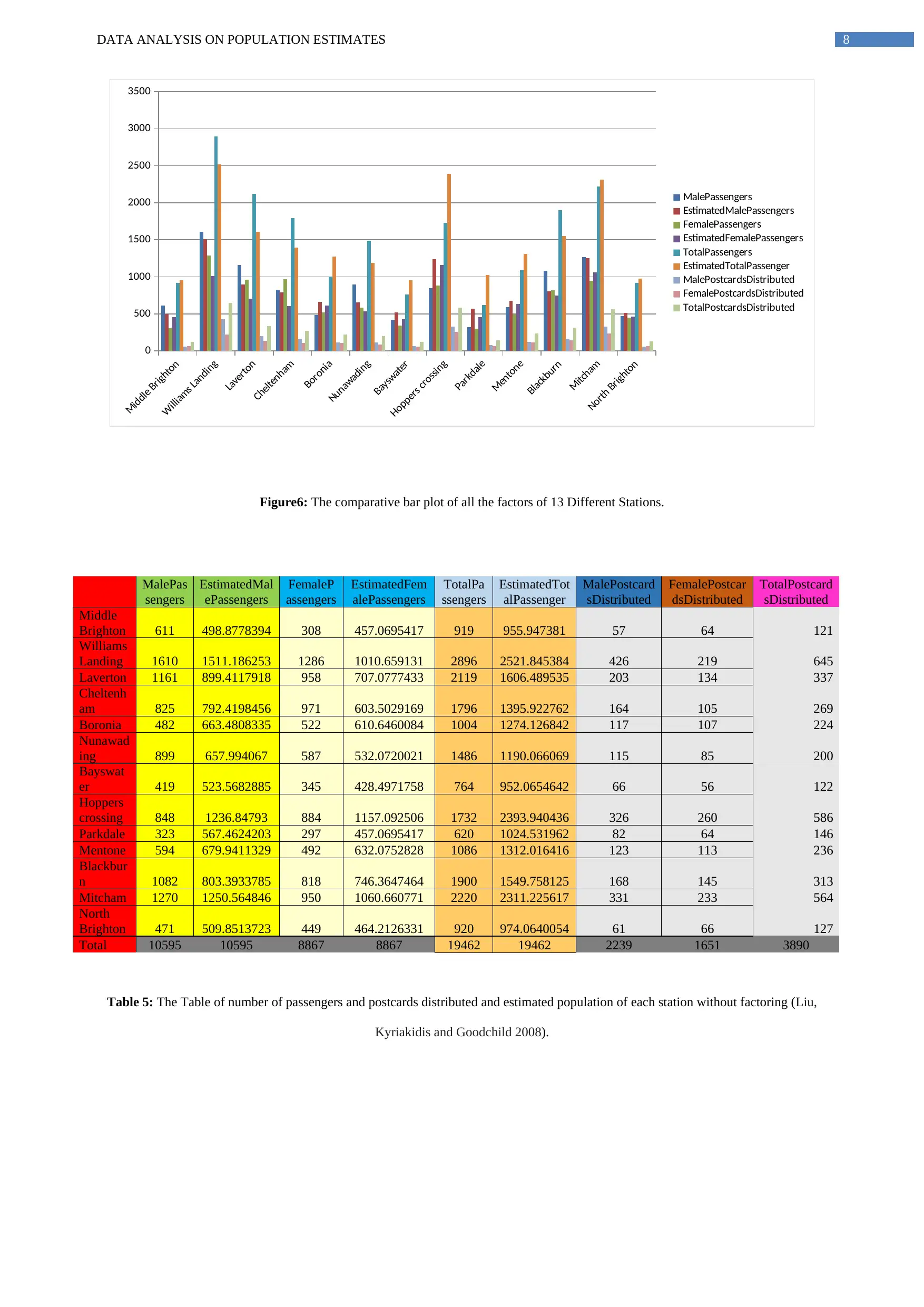
Figure6: The comparative bar plot of all the factors of 13 Different Stations.
MalePas
sengers
EstimatedMal
ePassengers
FemaleP
assengers
EstimatedFem
alePassengers
TotalPa
ssengers
EstimatedTot
alPassenger
MalePostcard
sDistributed
FemalePostcar
dsDistributed
TotalPostcard
sDistributed
Middle
Brighton 611 498.8778394 308 457.0695417 919 955.947381 57 64 121
Williams
Landing 1610 1511.186253 1286 1010.659131 2896 2521.845384 426 219 645
Laverton 1161 899.4117918 958 707.0777433 2119 1606.489535 203 134 337
Cheltenh
am 825 792.4198456 971 603.5029169 1796 1395.922762 164 105 269
Boronia 482 663.4808335 522 610.6460084 1004 1274.126842 117 107 224
Nunawad
ing 899 657.994067 587 532.0720021 1486 1190.066069 115 85 200
Bayswat
er 419 523.5682885 345 428.4971758 764 952.0654642 66 56 122
Hoppers
crossing 848 1236.84793 884 1157.092506 1732 2393.940436 326 260 586
Parkdale 323 567.4624203 297 457.0695417 620 1024.531962 82 64 146
Mentone 594 679.9411329 492 632.0752828 1086 1312.016416 123 113 236
Blackbur
n 1082 803.3933785 818 746.3647464 1900 1549.758125 168 145 313
Mitcham 1270 1250.564846 950 1060.660771 2220 2311.225617 331 233 564
North
Brighton 471 509.8513723 449 464.2126331 920 974.0640054 61 66 127
Total 10595 10595 8867 8867 19462 19462 2239 1651 3890
Table 5: The Table of number of passengers and postcards distributed and estimated population of each station without factoring (Liu,
Kyriakidis and Goodchild 2008).
Middle Brighton
Williams Landing
Laverton
Cheltenham
Boronia
Nunawading
Bayswater
Hoppers crossing
Parkdale
Mentone
Blackburn
Mitcham
North Brighton
0
500
1000
1500
2000
2500
3000
3500
MalePassengers
EstimatedMalePassengers
FemalePassengers
EstimatedFemalePassengers
TotalPassengers
EstimatedTotalPassenger
MalePostcardsDistributed
FemalePostcardsDistributed
TotalPostcardsDistributed
Figure6: The comparative bar plot of all the factors of 13 Different Stations.
MalePas
sengers
EstimatedMal
ePassengers
FemaleP
assengers
EstimatedFem
alePassengers
TotalPa
ssengers
EstimatedTot
alPassenger
MalePostcard
sDistributed
FemalePostcar
dsDistributed
TotalPostcard
sDistributed
Middle
Brighton 611 498.8778394 308 457.0695417 919 955.947381 57 64 121
Williams
Landing 1610 1511.186253 1286 1010.659131 2896 2521.845384 426 219 645
Laverton 1161 899.4117918 958 707.0777433 2119 1606.489535 203 134 337
Cheltenh
am 825 792.4198456 971 603.5029169 1796 1395.922762 164 105 269
Boronia 482 663.4808335 522 610.6460084 1004 1274.126842 117 107 224
Nunawad
ing 899 657.994067 587 532.0720021 1486 1190.066069 115 85 200
Bayswat
er 419 523.5682885 345 428.4971758 764 952.0654642 66 56 122
Hoppers
crossing 848 1236.84793 884 1157.092506 1732 2393.940436 326 260 586
Parkdale 323 567.4624203 297 457.0695417 620 1024.531962 82 64 146
Mentone 594 679.9411329 492 632.0752828 1086 1312.016416 123 113 236
Blackbur
n 1082 803.3933785 818 746.3647464 1900 1549.758125 168 145 313
Mitcham 1270 1250.564846 950 1060.660771 2220 2311.225617 331 233 564
North
Brighton 471 509.8513723 449 464.2126331 920 974.0640054 61 66 127
Total 10595 10595 8867 8867 19462 19462 2239 1651 3890
Table 5: The Table of number of passengers and postcards distributed and estimated population of each station without factoring (Liu,
Kyriakidis and Goodchild 2008).
⊘ This is a preview!⊘
Do you want full access?
Subscribe today to unlock all pages.
Trusted by 1+ million students worldwide

DATA ANALYSIS ON POPULATION ESTIMATES 9
Conclusion:-
The data analysis concludes that bicycle is the most uncommon transportation among all the transportation media to travel from home to
railway station. Employment is the key reason behind the trip. Generally, young generation prefers to travel than aged persons. It is found that
though body exercise and parking easiness are the major reasons for riding bicycles, but security concern, time taken and reliability in timing are
the main issues. The week association exists between distance covered and time elapsed due to travelling. Therefore, these two factors are not
highly related to each other. Few stations like Baywaster, Parkadale, Middle brighton and North brighton are not so popular in terms of total
population and postcard delivered. Government and Transport Corporation should look after that matter. The estimation of population in
different stations shows a good fitting (Henseler and Sarstedt 2013). The estimation is good fitted for following stations:
Male Passenger:
Williams Landing, Cheltenham, Bayswater, Mitcham, North Brighton, Mentone.
Female Passenger:
Boronia, Nunawading, Blackburn, Mitcham, North Brighton.
Total Passenger:
Middle Brighton, Mitcham, North Brighton.
Paraphrase This Document
Need a fresh take? Get an instant paraphrase of this document with our AI Paraphraser
DATA ANALYSIS ON POPULATION ESTIMATES 10
References:-
Darlington, R. B., & Hayes, A. F. (2016). Regression analysis and linear models: Concepts, applications, and implementation. Guilford
Publications.
Draper, N. R., & Smith, H. (2014). Applied regression analysis. John Wiley & Sons.
Henseler, J., & Sarstedt, M. (2013). Goodness-of-fit indices for partial least squares path modeling. Computational Statistics, 1-16.
Kahneman, D., Krueger, A.B., Schkade, D.A., Schwarz, N. and Stone, A.A., 2004. A survey method for characterizing daily life
experience: The day reconstruction method. Science, 306(5702), pp.1776-1780.
Salaria, N., 2012. Meaning of the term descriptive survey research method. International journal of transformations in business
management, 1(6), pp.161-175.
Good, I.J., 1953. The population frequencies of species and the estimation of population parameters. Biometrika, 40(3-4), pp.237-264.
Liu, X.H., Kyriakidis, P.C. and Goodchild, M.F., 2008. Population‐density estimation using regression and area‐to‐point residual
kriging. International Journal of geographical information science, 22(4), pp.431-447.
Lo, C.P., 2008. Population estimation using geographically weighted regression. GIScience & Remote Sensing, 45(2), pp.131-148.
1 out of 11
Your All-in-One AI-Powered Toolkit for Academic Success.
+13062052269
info@desklib.com
Available 24*7 on WhatsApp / Email
![[object Object]](/_next/static/media/star-bottom.7253800d.svg)
Unlock your academic potential
Copyright © 2020–2026 A2Z Services. All Rights Reserved. Developed and managed by ZUCOL.