Multi-Regression Analysis and Variable Selection

This assignment focuses on understanding multi-regression analysis and its application in predicting sales based on several factors. Students need to interpret regression results, identify significant predictors (X2, X4, X5), and discuss the implications of eliminating insignificant variables (X3, X6). The assignment involves analyzing provided tables containing regression coefficients, standard errors, t-statistics, p-values, and confidence intervals.

Data analysis 1
Title
Student’s name
Course title
Date

Data analysis 2
TASK ONE
Question 1
Summary statistics – capital
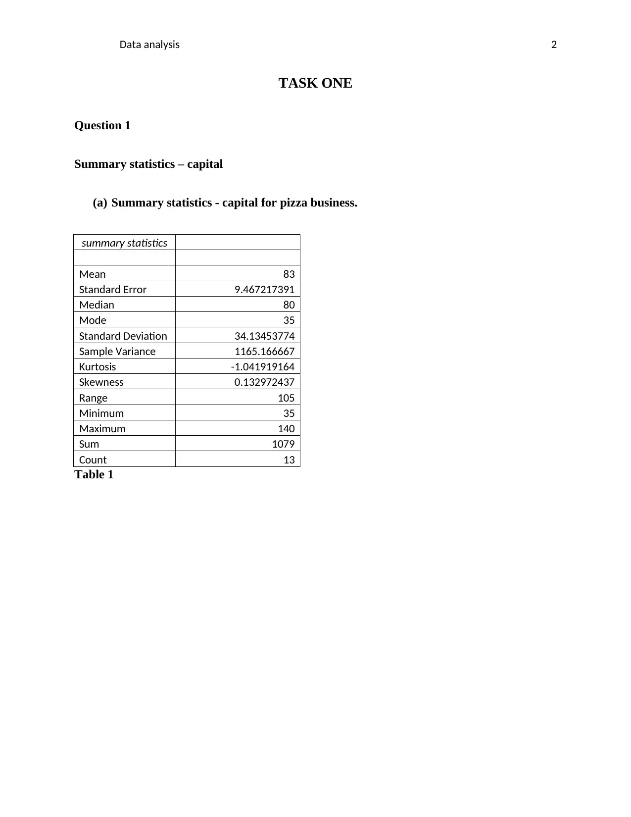
(a) Summary statistics - capital for pizza business.
summary statistics
Mean 83
Standard Error 9.467217391
Median 80
Mode 35
Standard Deviation 34.13453774
Sample Variance 1165.166667
Kurtosis -1.041919164
Skewness 0.132972437
Range 105
Minimum 35
Maximum 140
Sum 1079
Count 13
Table 1

Data analysis 3
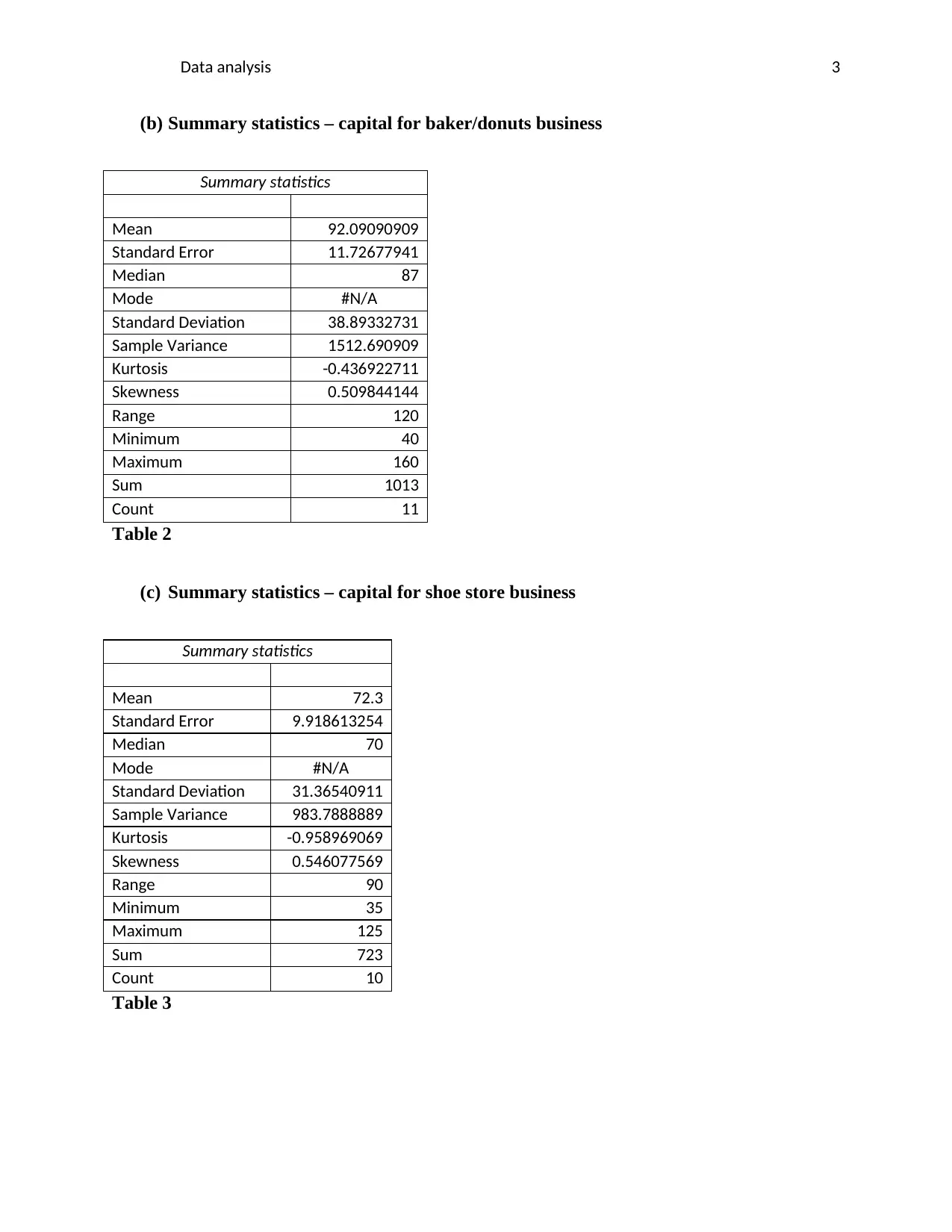
(b) Summary statistics – capital for baker/donuts business
Summary statistics
Mean 92.09090909
Standard Error 11.72677941
Median 87
Mode #N/A
Standard Deviation 38.89332731
Sample Variance 1512.690909
Kurtosis -0.436922711
Skewness 0.509844144
Range 120
Minimum 40
Maximum 160
Sum 1013
Count 11
Table 2
(c) Summary statistics – capital for shoe store business
Summary statistics
Mean 72.3
Standard Error 9.918613254
Median 70
Mode #N/A
Standard Deviation 31.36540911
Sample Variance 983.7888889
Kurtosis -0.958969069
Skewness 0.546077569
Range 90
Minimum 35
Maximum 125
Sum 723
Count 10
Table 3

Data analysis 4
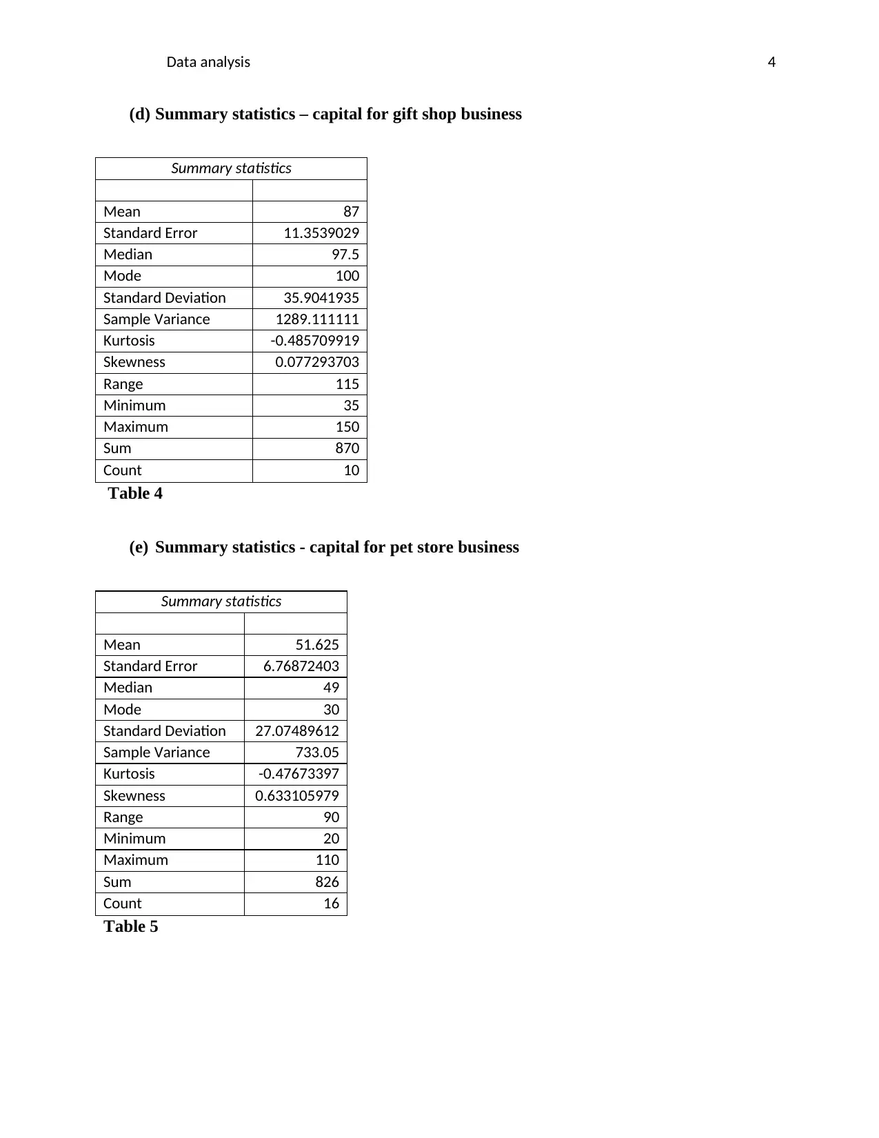
(d) Summary statistics – capital for gift shop business
Summary statistics
Mean 87
Standard Error 11.3539029
Median 97.5
Mode 100
Standard Deviation 35.9041935
Sample Variance 1289.111111
Kurtosis -0.485709919
Skewness 0.077293703
Range 115
Minimum 35
Maximum 150
Sum 870
Count 10
Table 4
(e) Summary statistics - capital for pet store business
Summary statistics
Mean 51.625
Standard Error 6.76872403
Median 49
Mode 30
Standard Deviation 27.07489612
Sample Variance 733.05
Kurtosis -0.47673397
Skewness 0.633105979
Range 90
Minimum 20
Maximum 110
Sum 826
Count 16
Table 5

Data analysis 5
Question 2
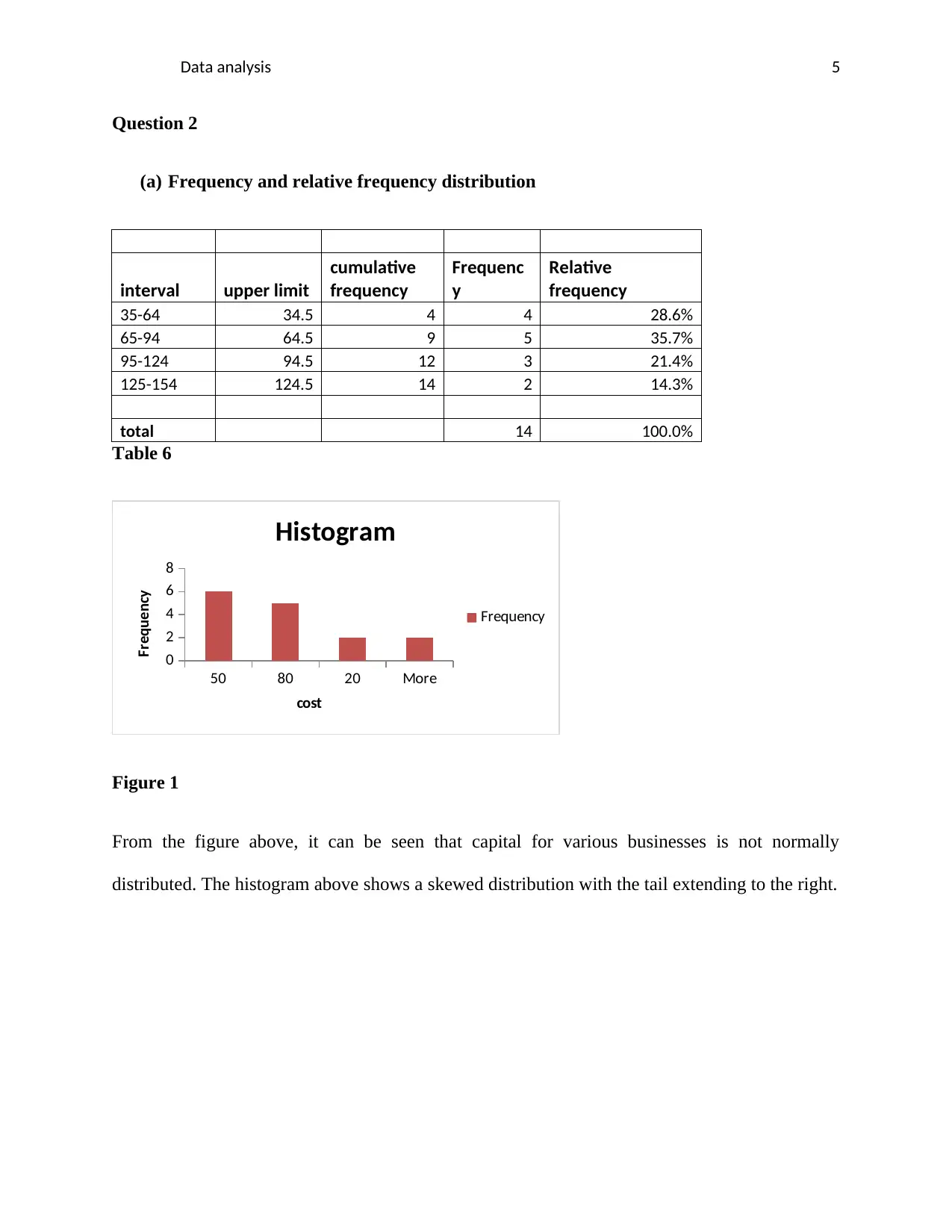
(a) Frequency and relative frequency distribution
interval upper limit
cumulative
frequency
Frequenc
y
Relative
frequency
35-64 34.5 4 4 28.6%
65-94 64.5 9 5 35.7%
95-124 94.5 12 3 21.4%
125-154 124.5 14 2 14.3%
total 14 100.0%
Table 6
50 80 20 More
0
2
4
6
8
Histogram
Frequency
cost
Frequency
Figure 1
From the figure above, it can be seen that capital for various businesses is not normally
distributed. The histogram above shows a skewed distribution with the tail extending to the right.

Data analysis 6
Question 3
Discussion
X1 X2 X3 X4 X5
Mean 83 Mean 92.090
9
Mean 72.3 Mean 87 Mean 51.625
Media
n
80 Media
n
87 Media
n
70 Media
n
97.5 Media
n
49
Mode 35 Mode #N/A Mode #N/A Mode 100 Mode 30
Std
Dev.
34.13
5
Std
Dev.
38.893
3
Std
Dev.
31.36
5
Std
Dev.
35.90
4
Std
Dev.
27.074
9
Var 1165.
2
Var 1512.6
9
Var 983.7
9
Var 1289.
1
Var 733.05
Range 105 Range 120 Range 90 Range 115 Range 90
Count 13 Count 11 Count 10 Count 10 Count 16
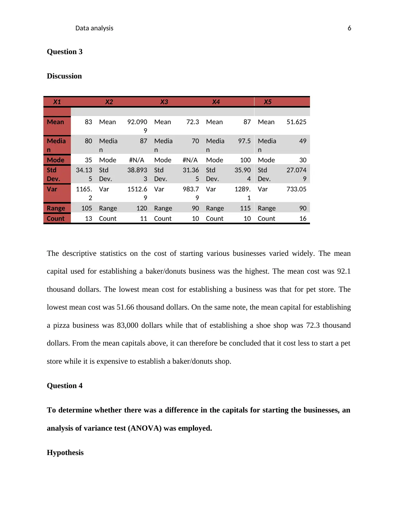
The descriptive statistics on the cost of starting various businesses varied widely. The mean
capital used for establishing a baker/donuts business was the highest. The mean cost was 92.1
thousand dollars. The lowest mean cost for establishing a business was that for pet store. The
lowest mean cost was 51.66 thousand dollars. On the same note, the mean capital for establishing
a pizza business was 83,000 dollars while that of establishing a shoe shop was 72.3 thousand
dollars. From the mean capitals above, it can therefore be concluded that it cost less to start a pet
store while it is expensive to establish a baker/donuts shop.
Question 4
To determine whether there was a difference in the capitals for starting the businesses, an
analysis of variance test (ANOVA) was employed.
Hypothesis

Data analysis 7
H0: There is no significant difference in the mean capital for the businesses.
Versus
H1: There is no significant difference in the mean capital for the businesses.
The test results are as tabulated in table 6 below;
SUMMARY
Groups Count Sum Average Varianc
e
X1 13 1079 83 1165.16
7
X2 11 1013 92.0909
1
1512.69
1
X3 10 723 72.3 983.788
9
X4 10 870 87 1289.11
1
X5 16 826 51.625 733.05
ANOVA
Source of
Variation
SS df MS F P-value F crit
Between Groups 14298.2
2
4 3574.55
6
3.24633
6
0.01839
1
2.53968
9
Within Groups 60560.7
6
55 1101.10
5
Total 74858.9
8
59
Table 6
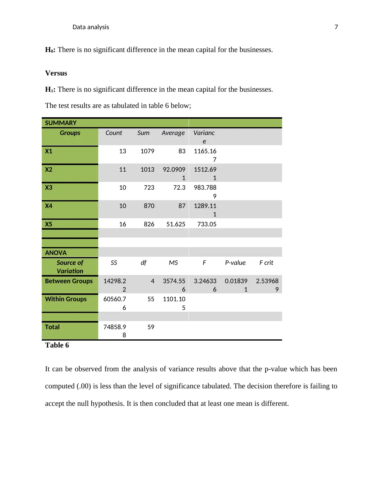
It can be observed from the analysis of variance results above that the p-value which has been
computed (.00) is less than the level of significance tabulated. The decision therefore is failing to
accept the null hypothesis. It is then concluded that at least one mean is different.

Data analysis 8
TASK TWO
Question 1
SUMMARY OUTPUT
Regression Statistics
Multiple R 0.996584
R Square 0.993179
Adjusted R
Square
0.991556
Standard
Error
17.64924
Observation
s
27
ANOVA
df SS MS F Significan
ce F
Regression 5 952538.9 19050 611.590 5.4E-22
Residual 21 6541.41 311.49
Total 26 959080.4
Coefficien
ts
Standard
Error
t Stat P-value Lower
95%
Upper
95%
Lower
95.0%
Upper
95.0%
Intercept -18.8594 30.15023 -
0.6255
1
0.53837
2
-81.5602 43.8414
2
-
81.5602
43.8414
2
X Variable 2 16.20157 3.544437 4.5709 0.00016 8.830513 23.5726 8.83051 23.5726
X Variable 3 0.174635 0.057606 3.0315 0.00634 0.054837 0.29443 0.05483 0.29443

Data analysis 9
X Variable 4 11.52627 2.532103 4.5520 0.00017 6.260472 16.7920 6.26047 16.7920
X Variable 5 13.58031 1.770457 7.6705 1.61E-0 9.898447 17.2621 9.89844 17.2621
X Variable 6 -5.31097 1.705427 -
3.1141
0.00524 -8.8576 -
1.76434
-8.8576 -
1.76434
Table 7
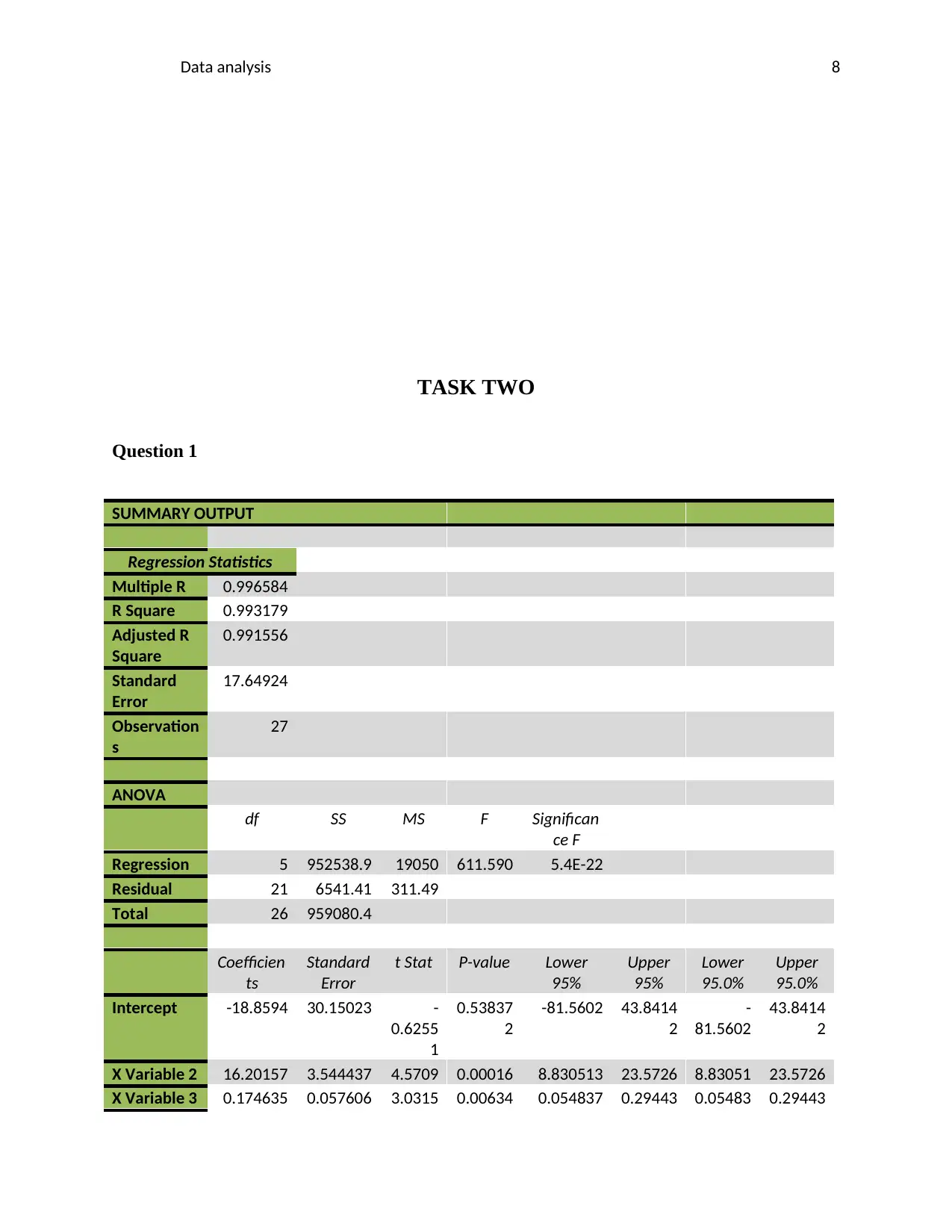
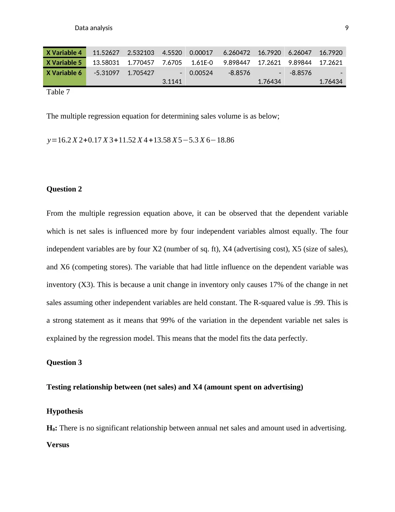
The multiple regression equation for determining sales volume is as below;
y=16.2 X 2+0.17 X 3+11.52 X 4 +13.58 X 5−5.3 X 6−18.86
Question 2
From the multiple regression equation above, it can be observed that the dependent variable
which is net sales is influenced more by four independent variables almost equally. The four
independent variables are by four X2 (number of sq. ft), X4 (advertising cost), X5 (size of sales),
and X6 (competing stores). The variable that had little influence on the dependent variable was
inventory (X3). This is because a unit change in inventory only causes 17% of the change in net
sales assuming other independent variables are held constant. The R-squared value is .99. This is
a strong statement as it means that 99% of the variation in the dependent variable net sales is
explained by the regression model. This means that the model fits the data perfectly.
Question 3
Testing relationship between (net sales) and X4 (amount spent on advertising)
Hypothesis
H0: There is no significant relationship between annual net sales and amount used in advertising.
Versus

Data analysis 10
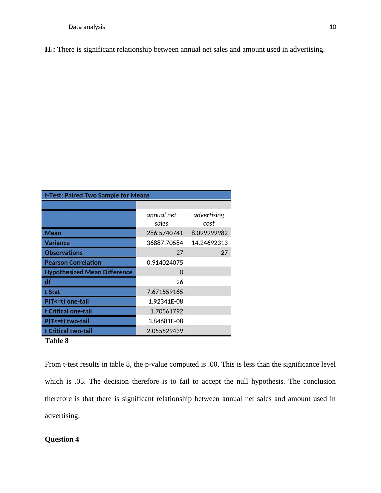
H1: There is significant relationship between annual net sales and amount used in advertising.
t-Test: Paired Two Sample for Means
annual net
sales
advertising
cost
Mean 286.5740741 8.099999982
Variance 36887.70584 14.24692313
Observations 27 27
Pearson Correlation 0.914024075
Hypothesized Mean Difference 0
df 26
t Stat 7.671559165
P(T<=t) one-tail 1.92341E-08
t Critical one-tail 1.70561792
P(T<=t) two-tail 3.84681E-08
t Critical two-tail 2.055529439
Table 8
From t-test results in table 8, the p-value computed is .00. This is less than the significance level
which is .05. The decision therefore is to fail to accept the null hypothesis. The conclusion
therefore is that there is significant relationship between annual net sales and amount used in
advertising.
Question 4

Data analysis 11
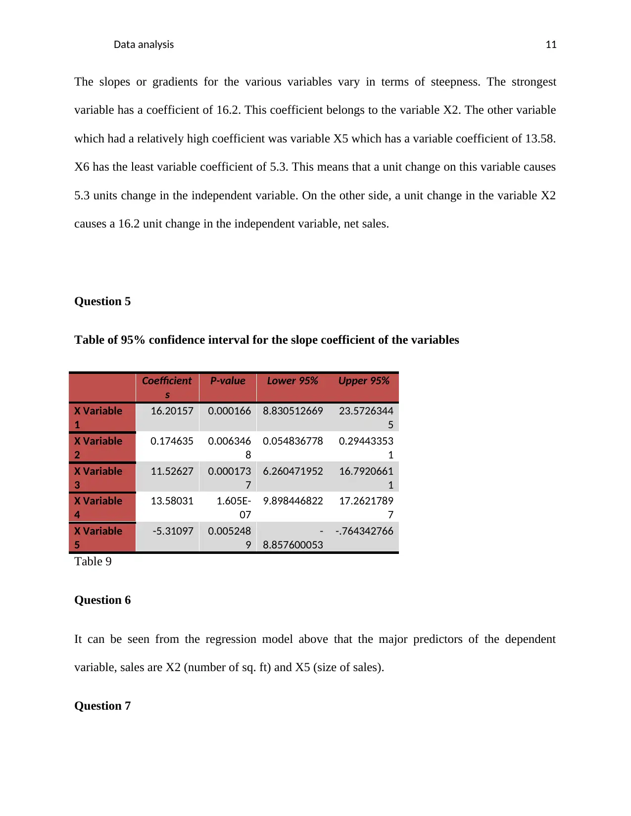
The slopes or gradients for the various variables vary in terms of steepness. The strongest
variable has a coefficient of 16.2. This coefficient belongs to the variable X2. The other variable
which had a relatively high coefficient was variable X5 which has a variable coefficient of 13.58.
X6 has the least variable coefficient of 5.3. This means that a unit change on this variable causes
5.3 units change in the independent variable. On the other side, a unit change in the variable X2
causes a 16.2 unit change in the independent variable, net sales.
Question 5
Table of 95% confidence interval for the slope coefficient of the variables
Coefficient
s
P-value Lower 95% Upper 95%
X Variable
1
16.20157 0.000166 8.830512669 23.5726344
5
X Variable
2
0.174635 0.006346
8
0.054836778 0.29443353
1
X Variable
3
11.52627 0.000173
7
6.260471952 16.7920661
1
X Variable
4
13.58031 1.605E-
07
9.898446822 17.2621789
7
X Variable
5
-5.31097 0.005248
9
-
8.857600053
-.764342766
Table 9
Question 6
It can be seen from the regression model above that the major predictors of the dependent
variable, sales are X2 (number of sq. ft) and X5 (size of sales).
Question 7

Data analysis 12
Coefficient
s
Standar
d Error
t Stat P-value Lower
95%
Upper
95%
Lower
95.0%
Upper
95.0%
Intercept -108.40792 10.3385 -
10.485
8
3.1E-10 -129.79 -87.021 -
129.79
5
-87.021
X Variable
2
20.571022 4.08328 5.0378
6
4.25E- 12.124 29.0179 12.124
1
29.0179
X Variable
4
19.086839 1.95871 9.7445
6
1.24E- 15.034 23.1387 15.034
9
23.1387
X Variable
5
17.741477 1.74783 10.150
5
5.76E-1 14.125
8
21.3571
6
14.125
8
21.3571
6
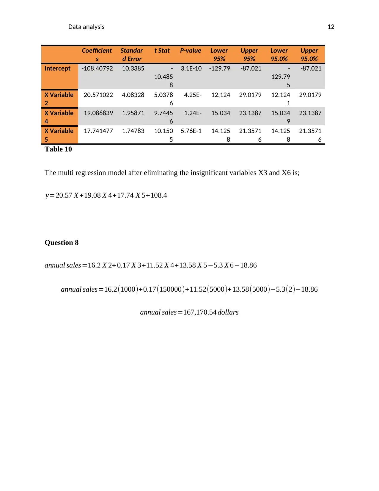
Table 10
The multi regression model after eliminating the insignificant variables X3 and X6 is;
y=20.57 X +19.08 X 4+17.74 X 5+108.4
Question 8
annual sales=16.2 X 2+ 0.17 X 3+11.52 X 4+13.58 X 5−5.3 X 6−18.86
annual sales=16.2(1000)+0.17(150000)+11.52(5000)+ 13.58(5000)−5.3(2)−18.86
annual sales=167,170.54 dollars