Data Analysis report of Road Crashes
VerifiedAdded on 2023/03/31
|13
|2045
|350
AI Summary
This report presents the analysis of road accidents from 1989 to 2019 using techniques like cluster analysis and linear regression analysis. The data contains mostly qualitative data and can be used for further advanced studies. The report describes the data using one variable analysis and two variable analysis.
Contribute Materials
Your contribution can guide someone’s learning journey. Share your
documents today.

Data Analysis report of Road Crashes from 1989 to 2019
Name of the Student:
Name of the University:
Author Note:
Name of the Student:
Name of the University:
Author Note:
Secure Best Marks with AI Grader
Need help grading? Try our AI Grader for instant feedback on your assignments.

Table of Contents
Introduction...............................................................................................................................2
Data setup..................................................................................................................................2
Explanatory Data Analysis..........................................................................................................2
One variable Analysis “AGE”..................................................................................................2
One variable Analysis “SPEED LIMIT”.....................................................................................4
Two Variable Analysis............................................................................................................5
Two variable analysis “GENDER & CRASH TYPE”...............................................................5
Two variable analysis “CRASH TYPE & ROAD USER”..........................................................5
Advanced Analysis......................................................................................................................6
Clustering...............................................................................................................................6
Concept of k-means Cluster Analysis.................................................................................6
Clustering Analysis.............................................................................................................6
Linear regression Analysis......................................................................................................9
Conclusion................................................................................................................................10
Reflections................................................................................................................................10
Reference and Bibliography:....................................................................................................12
Page 1
Data analysis report of road crashes from 1989 to 2019

Introduction
The report presents the analysis of road accidents form 1989 to 2019. There are
techniques like cluster analysis and linear regression analysis which are used here. The data
contains mostly qualitative data and these can be used for further advance studies like
prediction of speed limit that encourages multiple crashes (Cox 2018). The paper describes
the data using one variable analysis and two variable analysis. The data is available on the
Australian government website. Excel is used to clean and R is used to perform the analysis.
Data setup
The data file used in the analysis was copied in a new excel workbook and saved as
xlsx file. The data was then edited by using EXCEL 2013 where the observations were
deleted which contains the value -9 as it indicates missing value and unknown information.
After cleaning the data xlsx file was uploaded in the R workspace for further steps towards
analysis. The command used to upload the file is mentioned below:
Uploading data file: crash <- readxl::read_xlsx(file.choose())
There are three libraries that were loaded for the analysis. The libraries are “stats”,
“RColorBrewer” and “ggplot2” for statistical functions and data visualisation.
library(stats)
library(RColorBrewer)
library(ggplot2)
Before going to the analysis part, the initial step was to remove the missing values
from the data set which were automatically assigned as NA. The following command was
used to omit the NA values from the data set.
na.omit(mydata$`Crash Type`)
na.omit(mydata$`Bus Involvement`)
na.omit(mydata$`Articulated Truck Involvement`)
na.omit(mydata$`Speed Limit`)
na.omit(mydata$`Road User`)
na.omit(mydata$Gender)
na.omit(mydata$Age)
The above commands ensures that the further steps were not going to be disturbed
by the missing values. Hence, the analysis proceeded for the one variable analysis and so on.
Explanatory Data Analysis
One variable Analysis “AGE”
summary(mydata$Age)
boxplot(mydata$Age,col = "blue")
Page 2
Data analysis report of road crashes from 1989 to 2019

Figure 1: Histogram of Age
The figure 1 presents the frequency distribution of age and the shape of distribution
which is left skewed. The table 1 shows the average age of the observed sample which is 41.
The quartiles are presented by the box plot too.
Table 1: Summary statistics of age
Figure 2: Box plot of age
The figure 2 and table 1 presents the lower upper quartile which is 23 and 57
respectively. The additional feature of the box plot is showing the outliers which is not
present in the age variable (Wickham 2016).
Page 3
Data analysis report of road crashes from 1989 to 2019
Secure Best Marks with AI Grader
Need help grading? Try our AI Grader for instant feedback on your assignments.

One variable Analysis “SPEED LIMIT”
hist(mydata$`Speed Limit`,col = "green")
summary(mydata$`Speed Limit`)
Figure 3: Histogram of speed limit
The figure 3 presents the histogram for the frequency distribution for the speed limit
which is uneven. The histogram shows that the most of the individuals’ speed limit is around
100. The table 2 presents the average speed limit that is 82.93.
Table 2: Summary statistics of speed limit
The lower quartile and the upper quartile of speed limit is 60 and 100 which means
most of the people drive with a speed limit that ranges between 60 and 100. This is
presented in the box plot of speed limit.
Figure 4: Boxplot for the speed limit
Page 4
Data analysis report of road crashes from 1989 to 2019
Two Variable Analysis
Two variable analysis “GENDER & CRASH TYPE”
GenderCrash<- table(mydata$Gender,mydata$`Crash Type`)
barplot(table(mydata$Gender),col="yellow")
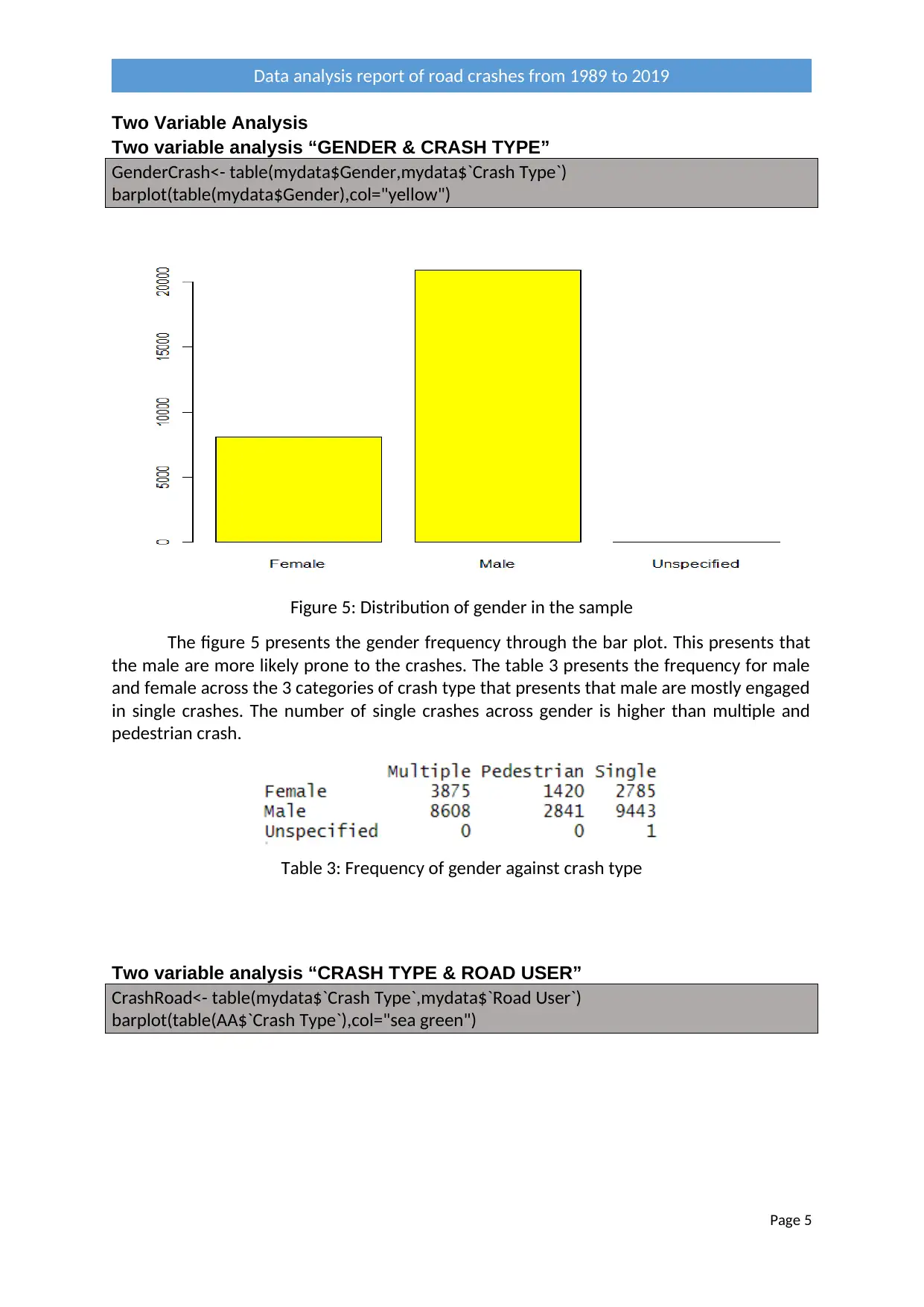
Figure 5: Distribution of gender in the sample
The figure 5 presents the gender frequency through the bar plot. This presents that
the male are more likely prone to the crashes. The table 3 presents the frequency for male
and female across the 3 categories of crash type that presents that male are mostly engaged
in single crashes. The number of single crashes across gender is higher than multiple and
pedestrian crash.
Table 3: Frequency of gender against crash type
Two variable analysis “CRASH TYPE & ROAD USER”
CrashRoad<- table(mydata$`Crash Type`,mydata$`Road User`)
barplot(table(AA$`Crash Type`),col="sea green")
Page 5
Data analysis report of road crashes from 1989 to 2019
Two variable analysis “GENDER & CRASH TYPE”
GenderCrash<- table(mydata$Gender,mydata$`Crash Type`)
barplot(table(mydata$Gender),col="yellow")
Figure 5: Distribution of gender in the sample
The figure 5 presents the gender frequency through the bar plot. This presents that
the male are more likely prone to the crashes. The table 3 presents the frequency for male
and female across the 3 categories of crash type that presents that male are mostly engaged
in single crashes. The number of single crashes across gender is higher than multiple and
pedestrian crash.
Table 3: Frequency of gender against crash type
Two variable analysis “CRASH TYPE & ROAD USER”
CrashRoad<- table(mydata$`Crash Type`,mydata$`Road User`)
barplot(table(AA$`Crash Type`),col="sea green")
Page 5
Data analysis report of road crashes from 1989 to 2019

Figure 6: Distribution of crash type in the sample
The figure 6 presents the crash type frequency through the bar plot. This presents
that the single and multiple crashes are more likely. The table 4 presents the frequency for
crash types across the categories of road users that presents that drivers are mostly
engaged in single and multiple crashes. The number of single crashes is higher than multiple
crashes for the driver where it is lower in case off motorcycle pillion passenger and
motorcycle rider.
Table 4: Frequency of crash against road user
Advanced Analysis
Clustering
Concept of k-means Cluster Analysis
K means clustering separates n number of observations into k number of clusters
with the nearest mean value of the k cluster (Cohen et al. 2015). The cluster contains the
observations that has similar mean and the different cluster contains the observations that
has different mean from other observations belongs to the other cluster. In k means
method, Euclidean distance is presented as metric and the variance is presented as the
measure of scatter of cluster (Shukri et al. 2018). The k is set manually so it is important to
follow proper process to determine the k or conduct a test for the specific value of k to
check the reliability of the k, otherwise the cluster analysis will not be able to perform well.
Clustering Analysis
The wssplot function is generated to plot the wss to determine the numbers of
cluster (Kassambara 2017). The required command is mentioned below:
wssplot<- function(data, nc=15,seed=1234)
#To determine the optimal number of cluster.
{
wss<- (nrow(data)-1)*sum(apply(data,2,var))
Page 6
Data analysis report of road crashes from 1989 to 2019
Paraphrase This Document
Need a fresh take? Get an instant paraphrase of this document with our AI Paraphraser
for(i in 2:nc){
set.seed(seed)
wss[i]<-sum(kmeans(data,centers = i)$withinss)
}
plot(1:nc,wss,type="b",xlab="Numbber of Clusters",
ylab="within groups sum of squares")
}
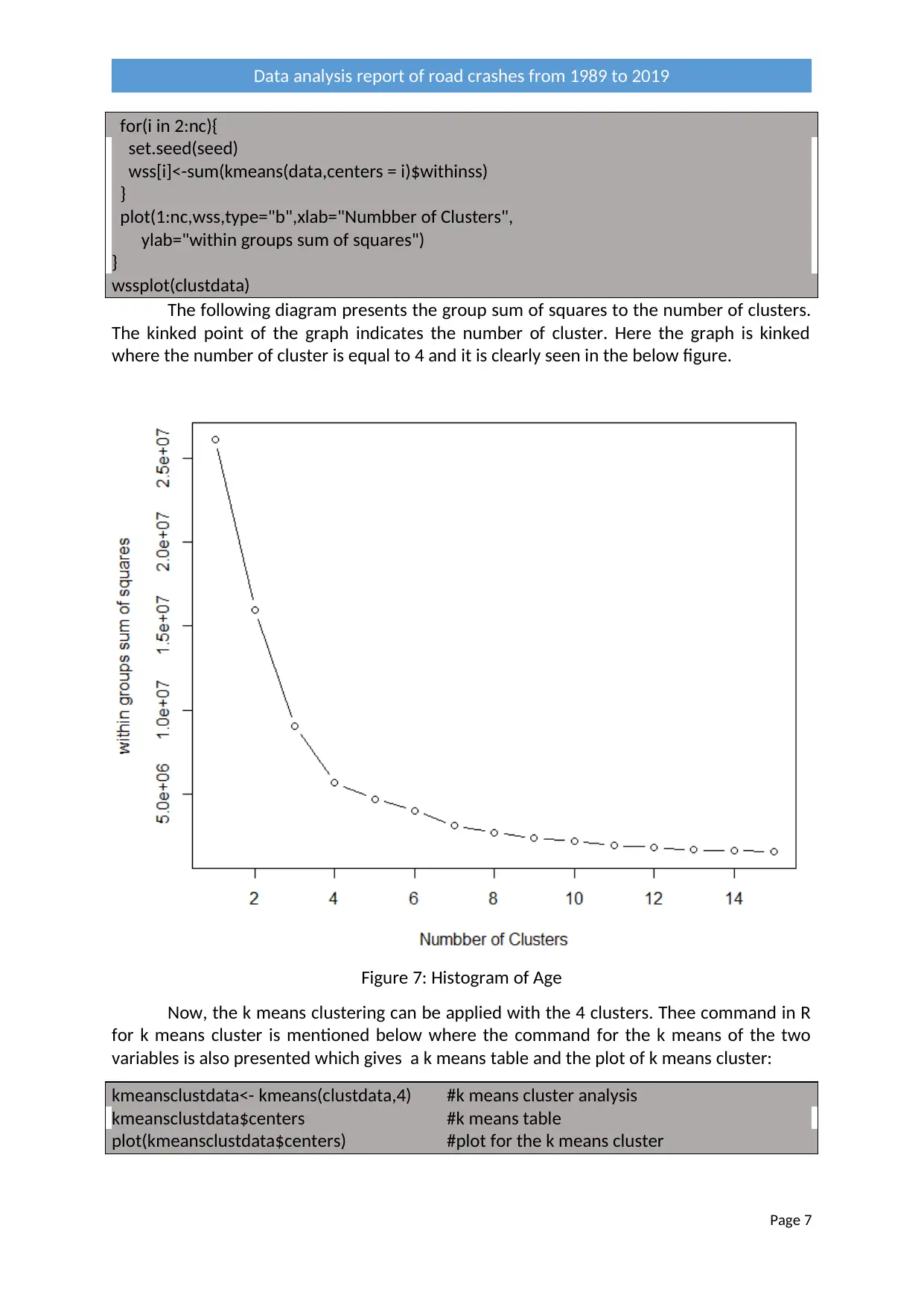
wssplot(clustdata)
The following diagram presents the group sum of squares to the number of clusters.
The kinked point of the graph indicates the number of cluster. Here the graph is kinked
where the number of cluster is equal to 4 and it is clearly seen in the below figure.
Figure 7: Histogram of Age
Now, the k means clustering can be applied with the 4 clusters. Thee command in R
for k means cluster is mentioned below where the command for the k means of the two
variables is also presented which gives a k means table and the plot of k means cluster:
kmeansclustdata<- kmeans(clustdata,4) #k means cluster analysis
kmeansclustdata$centers #k means table
plot(kmeansclustdata$centers) #plot for the k means cluster
Page 7
Data analysis report of road crashes from 1989 to 2019
set.seed(seed)
wss[i]<-sum(kmeans(data,centers = i)$withinss)
}
plot(1:nc,wss,type="b",xlab="Numbber of Clusters",
ylab="within groups sum of squares")
}
wssplot(clustdata)
The following diagram presents the group sum of squares to the number of clusters.
The kinked point of the graph indicates the number of cluster. Here the graph is kinked
where the number of cluster is equal to 4 and it is clearly seen in the below figure.
Figure 7: Histogram of Age
Now, the k means clustering can be applied with the 4 clusters. Thee command in R
for k means cluster is mentioned below where the command for the k means of the two
variables is also presented which gives a k means table and the plot of k means cluster:
kmeansclustdata<- kmeans(clustdata,4) #k means cluster analysis
kmeansclustdata$centers #k means table
plot(kmeansclustdata$centers) #plot for the k means cluster
Page 7
Data analysis report of road crashes from 1989 to 2019

The below table shows the cluster means that is generated from the cluster analysis.
The table shows 4 cluster means for each variable. This implies that in 1st cluster the average
speed and average age is 64.65 and 27.103 respectively.
Table 5: Cluster means of speed limit and age
The below figure presents 4 points for 4 clusters which represents that the
observations will be close to these points or the points are the mean of speed limit across
average age of each cluster.
Figure 8: Cluster mean plot of speed limit and age
Page 8
Data analysis report of road crashes from 1989 to 2019

Linear regression Analysis
Linear regression presents the relation between two or more variable where a
variable is dependent and the other variables are independent (Berger, Maurer and Celli
2018). The linear model is presented is as below:
Y=a + b*X
Where Y is the dependent variable and X is independent variable. The “a” is the
intercept term and “b” is the intercept term of the model. This parameters have their own
interpretation. The intercept term presents the value of Y when X is zero and the slope term
presents the change in Y due to one unit of change in X. This analysis is mainly used to check
find relation between variables and to predict the dependent variable.
x=1:28973 # X is assigned as the age
y=clustdata$`Speed Limit` #Y is assigned as the speed limit
linearreg<-lm(y~x) # linear regression
summary(linearreg) #Regression Result
abline(linearreg,col="green",lty=2, lwd=2) #Plot for the estimated trend line
The regression result is presented using the summary function in the following table
where the residuals summary statistics, estimated coefficients and corresponding standard
error and p-value, adjusted R2 and F-stat is available (Faraway 2016). The coefficients
standard errors and the p-values are very small which indicates that the coefficients are
statistically significant with minimum error. F-statistics is F (28971, 0.0094) = 6.74 is
significant that indicates the model is significant with the variables (Hanley 2016). However
the R2 is 0.00023 which is very small that says the goodness of fit of the model is worse or
the age cannot explain the speed limit.
Table 6: Regression Result
The eestimated regression equation is presented in the below figure which is in
green colour showing a linear relation between age and speed limit. The intercept and the
slope of the trendline is significant.
Page 9
Data analysis report of road crashes from 1989 to 2019
Secure Best Marks with AI Grader
Need help grading? Try our AI Grader for instant feedback on your assignments.

Figure 9: Trend line obtained from the regression
Conclusion
The variables age and speed limit is described through the one variable analysis
where the location of variables through mean, shape of the variables through histogram and
the outliers through boxplot is presented. Gender vs. crash type and crash type vs. road
users is described through two variable analysis where the frequency is presented for
gender against crash type and the crash type against road users. The conclusion from two
variable analysis says that male are most likely to engage in crashes and the males engage in
single crashes mostly. Most of the road users are driver who engage in crash and they
mostly engage in single crash. The linear regression analysis presents a significant relation
between age and speed limit. However the model cannot be used to predict the speed limit
for a specific age.
Reflections
The cluster analysis groups the observations in 4 clusters here. The wssplot helped to
determine the number of optimum clusters. Statistical techniques are used for qualitative
and quantitative analysis and also used for the prediction. The data set used in this analysis
is mostly qualitative and this paper is focused on the quantitative analysis. Hence there is a
lot to analyse. For example, a logit and tobit model can be used for the binary response
variables and ordered response variables. The binary response variable in this model is
gender and the ordered response variable is crash type.
Page 10
Data analysis report of road crashes from 1989 to 2019

Page 11
Data analysis report of road crashes from 1989 to 2019
Data analysis report of road crashes from 1989 to 2019

Reference and Bibliography:
Berger, P.D., Maurer, R.E. and Celli, G.B., 2018. Introduction to Simple Regression.
In Experimental Design (pp. 483-503). Springer, Cham.
Cohen, M.B., Elder, S., Musco, C., Musco, C. and Persu, M., 2015, June. Dimensionality
reduction for k-means clustering and low rank approximation. In Proceedings of the forty-
seventh annual ACM symposium on Theory of computing (pp. 163-172). ACM.
Cox, D.R., 2018. Analysis of binary data. Routledge.
Faraway, J.J., 2016. Linear models with R. Chapman and Hall/CRC.
Hanley, J.A., 2016. Simple and multiple linear regression: sample size considerations. Journal
of clinical epidemiology, 79, pp.112-119.
Kassambara, A., 2017. Practical guide to cluster analysis in R: unsupervised machine
learning (Vol. 1). STHDA.
Lem, S., Onghena, P., Verschaffel, L. and Van Dooren, W., 2017. The power of refutational
text: changing intuitions about the interpretation of box plots. European Journal of
Psychology of Education, 32(4), pp.537-550.
Neuendorf, K.A., 2016. The content analysis guidebook. Sage.
Shukri, S., Faris, H., Aljarah, I., Mirjalili, S. and Abraham, A., 2018. Evolutionary static and
dynamic clustering algorithms based on multi-verse optimizer. Engineering Applications of
Artificial Intelligence, 72, pp.54-66.
Wickham, H., 2016. ggplot2: elegant graphics for data analysis. Springer.
Page 12
Data analysis report of road crashes from 1989 to 2019
1 out of 13
Related Documents


Your All-in-One AI-Powered Toolkit for Academic Success.
+13062052269
info@desklib.com
Available 24*7 on WhatsApp / Email
![[object Object]](/_next/static/media/star-bottom.7253800d.svg)
Unlock your academic potential
© 2024 | Zucol Services PVT LTD | All rights reserved.