Analysis of Australian Road Fatalities - USC, Queensland, 2019
VerifiedAdded on 2023/03/30
|16
|1986
|225
Report
AI Summary
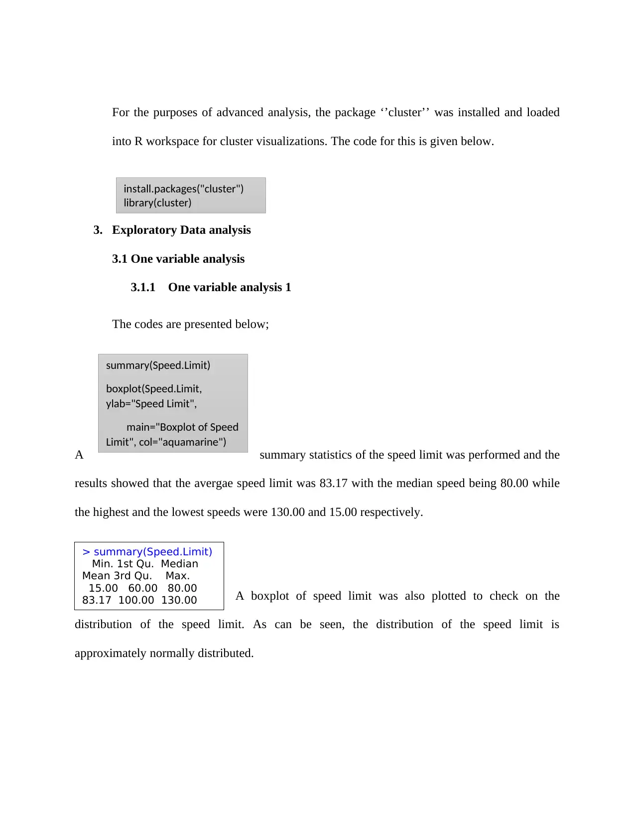
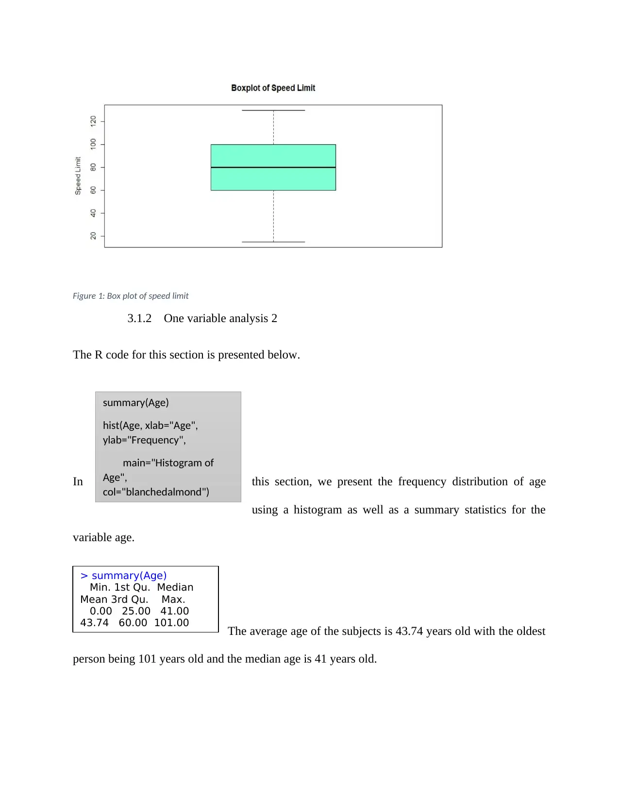
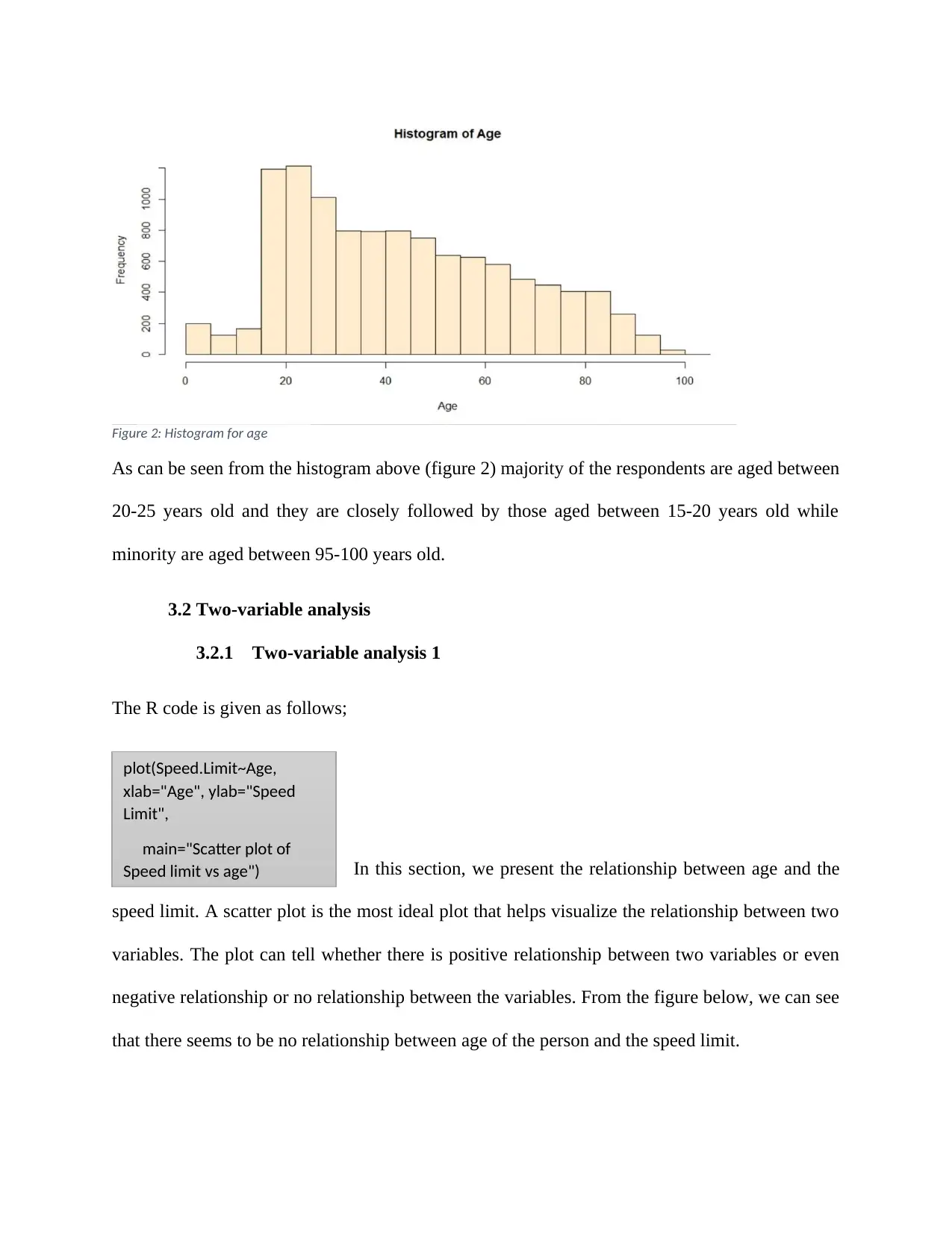
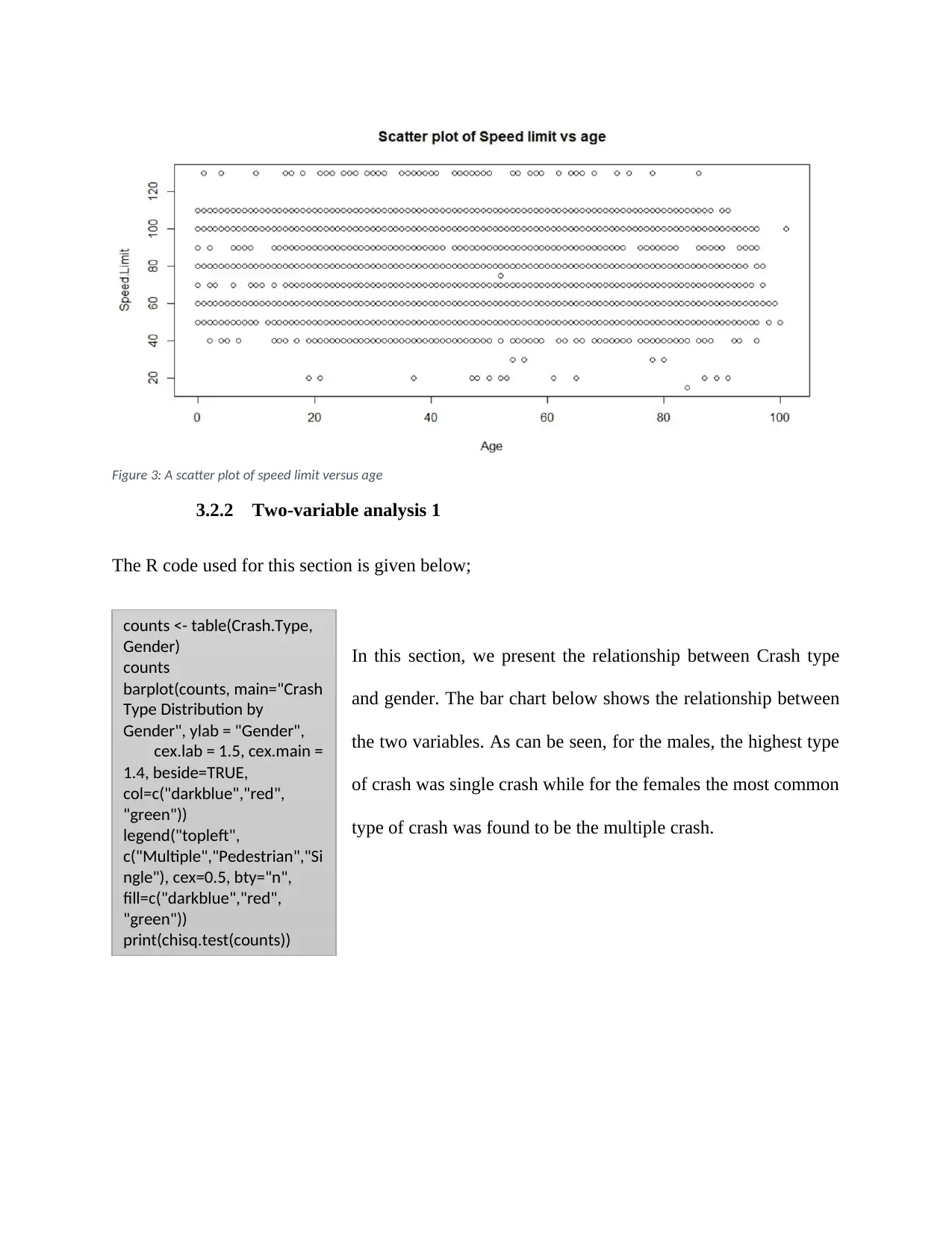
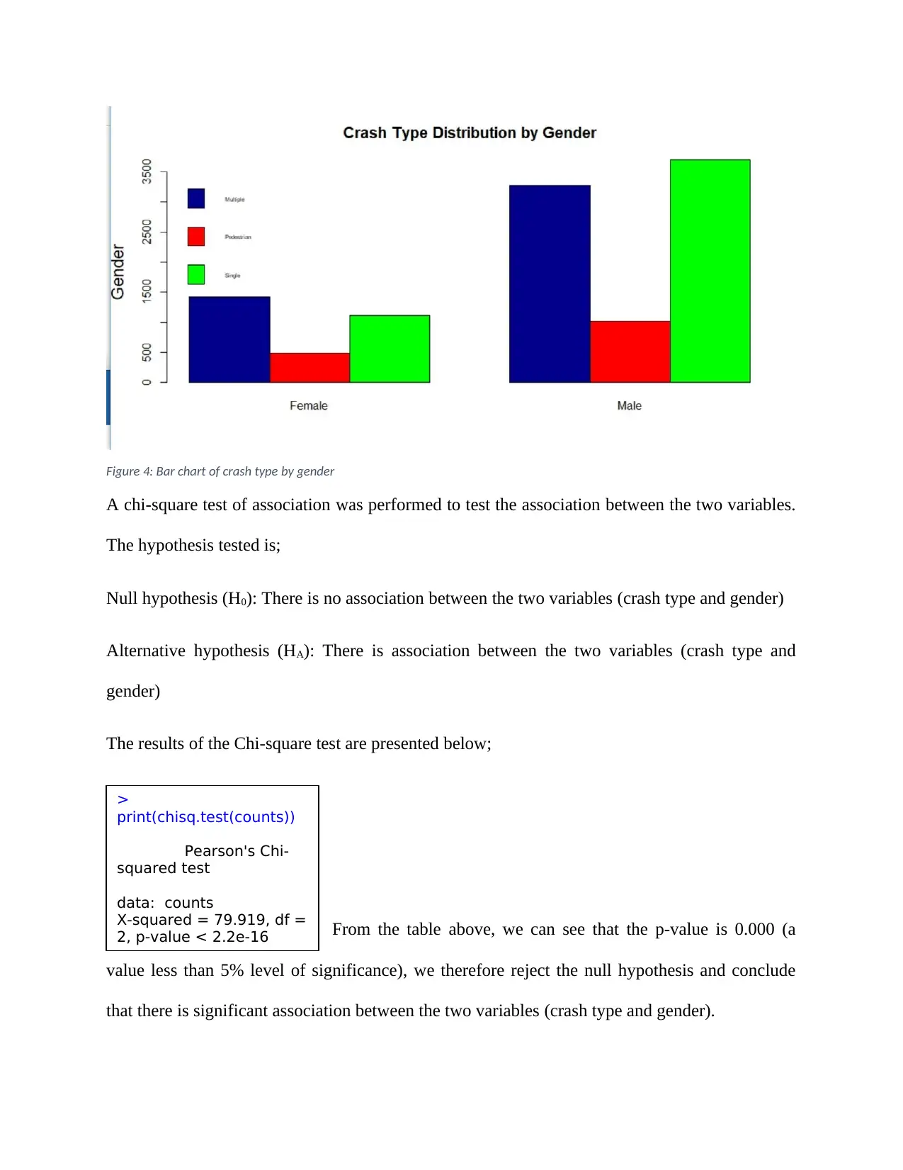
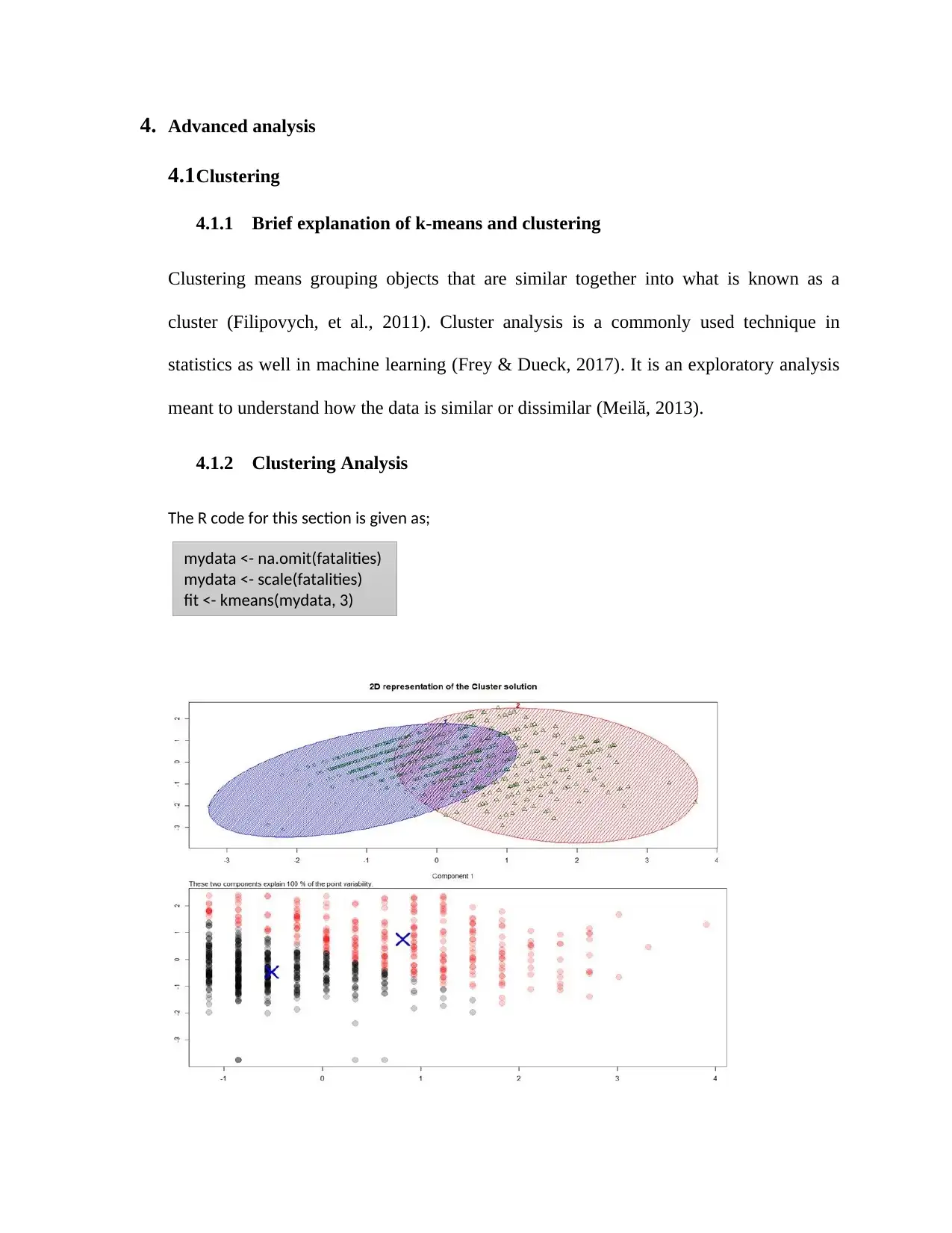
This data analysis report investigates fatality trends across six Australian states and two territories using data from the World Bank database. The analysis includes data pre-processing, cleaning, one and two-variable analyses, cluster analysis, and regression analysis with plots. Key findings include the average speed limit being 83.17, with a median of 80.00. The majority of fatalities involved individuals aged 15-25. A significant association was found between crash type and gender, while no direct relationship was observed between speed limit and age. Regression analysis indicated that gender significantly predicts speed limit, with males likely having lower speed limits than females. The report concludes by reflecting on the skills utilized, emphasizing the importance of data cleaning and modeling. Desklib provides access to similar reports and solved assignments for students.
1 out of 16
Related Documents


Your All-in-One AI-Powered Toolkit for Academic Success.
+13062052269
info@desklib.com
Available 24*7 on WhatsApp / Email
![[object Object]](/_next/static/media/star-bottom.7253800d.svg)
Copyright © 2020–2026 A2Z Services. All Rights Reserved. Developed and managed by ZUCOL.