Data Analysis Report

This data analysis report provides statistical analysis and interpretation of various factors. It includes t-tests, regression analysis, and correlation analysis to determine relationships between variables. The report covers topics such as mean values, variances, hypothesis testing, and significance levels. It also includes interpretations and conclusions based on the analysis. Download the report for a detailed understanding of the data.

Data Analysis Report

Table of Contents
Question 1........................................................................................................................................2
Question 2........................................................................................................................................2
Question 3........................................................................................................................................3
Question 4........................................................................................................................................3

Question 1
a)
t-Test: Two-Sample Assuming Unequal Variances
2 4
Mean 3.028228652 1.947776994
Variance 1.663044388 1.20631038
Observations 1417 1417
Hypothesized Mean Difference 0
df 2762
t Stat 24.01033069
P(T<=t) one-tail
3.69017017886002
E-116
t Critical one-tail 1.645405504
P(T<=t) two-tail 7.38E-116
t Critical two-tail 1.960823199
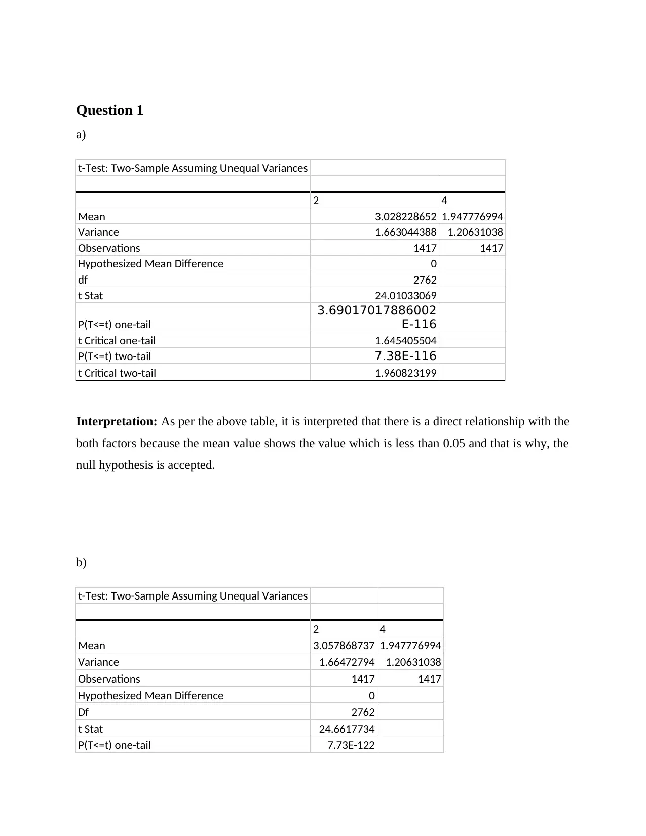
Interpretation: As per the above table, it is interpreted that there is a direct relationship with the
both factors because the mean value shows the value which is less than 0.05 and that is why, the
null hypothesis is accepted.
b)
t-Test: Two-Sample Assuming Unequal Variances
2 4
Mean 3.057868737 1.947776994
Variance 1.66472794 1.20631038
Observations 1417 1417
Hypothesized Mean Difference 0
Df 2762
t Stat 24.6617734
P(T<=t) one-tail 7.73E-122

t Critical one-tail 1.645405504
P(T<=t) two-tail 1.55E-121
t Critical two-tail 1.960823199
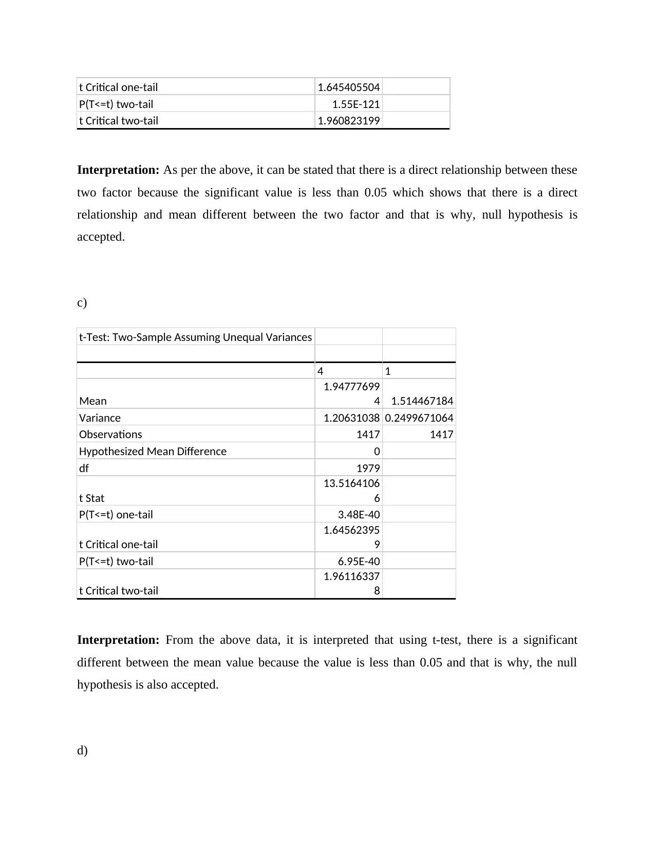
Interpretation: As per the above, it can be stated that there is a direct relationship between these
two factor because the significant value is less than 0.05 which shows that there is a direct
relationship and mean different between the two factor and that is why, null hypothesis is
accepted.
c)
t-Test: Two-Sample Assuming Unequal Variances
4 1
Mean
1.94777699
4 1.514467184
Variance 1.20631038 0.2499671064
Observations 1417 1417
Hypothesized Mean Difference 0
df 1979
t Stat
13.5164106
6
P(T<=t) one-tail 3.48E-40
t Critical one-tail
1.64562395
9
P(T<=t) two-tail 6.95E-40
t Critical two-tail
1.96116337
8
Interpretation: From the above data, it is interpreted that using t-test, there is a significant
different between the mean value because the value is less than 0.05 and that is why, the null
hypothesis is also accepted.
d)

t-Test: Two-Sample Assuming Unequal Variances
4 4
Mean 2.196894848 3.899788285
Variance 1.221798261 5.174978769
Observations 1417 1417
Hypothesized Mean Difference 0
df 2049
t Stat
-
25.34497052
P(T<=t) one-tail 8.37E-124
t Critical one-tail 1.645597631
P(T<=t) two-tail 1.67E-123
t Critical two-tail 1.961122377
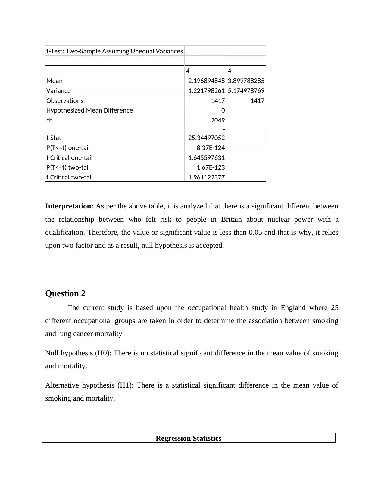
Interpretation: As per the above table, it is analyzed that there is a significant different between
the relationship between who felt risk to people in Britain about nuclear power with a
qualification. Therefore, the value or significant value is less than 0.05 and that is why, it relies
upon two factor and as a result, null hypothesis is accepted.
Question 2
The current study is based upon the occupational health study in England where 25
different occupational groups are taken in order to determine the association between smoking
and lung cancer mortality
Null hypothesis (H0): There is no statistical significant difference in the mean value of smoking
and mortality.
Alternative hypothesis (H1): There is a statistical significant difference in the mean value of
smoking and mortality.
Regression Statistics

Multiple R 0.7162398
R Square 0.51299945
Adjusted R Square 0.49182552
Standard Error 18.6153875
Observations 25
ANOVA
df SS MS F
Significance
F
Regression 1 8395.74904 8395.74904 24.227873 5.6576E-05
Residual 23 7970.25096 346.53265
Total 24 16366
Coeffici
ents
Standard
Error t Stat P-value
Lower
95%
Upper
95%
Lower
95.0%
Upper
95.0%
Interc
ept
-
2.88531
89
23.033721
6
-
0.12526
5
0.90140
224
-
50.5342
02
44.7635
644
-
50.53420
2
44.7635
644
Smok
ing
1.08753
226
0.2209451
7
4.92218
173
5.6576
E-05
0.63047
236
1.54459
216
0.630472
36
1.54459
216
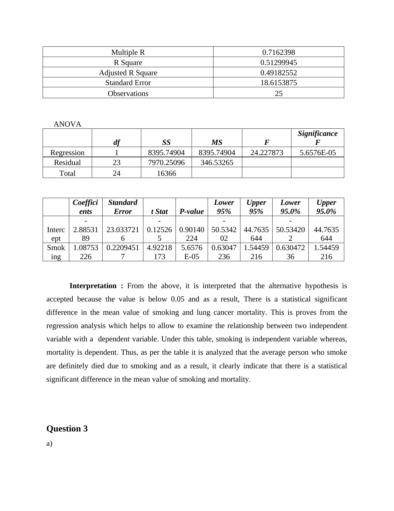
Interpretation : From the above, it is interpreted that the alternative hypothesis is
accepted because the value is below 0.05 and as a result, There is a statistical significant
difference in the mean value of smoking and lung cancer mortality. This is proves from the
regression analysis which helps to allow to examine the relationship between two independent
variable with a dependent variable. Under this table, smoking is independent variable whereas,
mortality is dependent. Thus, as per the table it is analyzed that the average person who smoke
are definitely died due to smoking and as a result, it clearly indicate that there is a statistical
significant difference in the mean value of smoking and mortality.
Question 3
a)

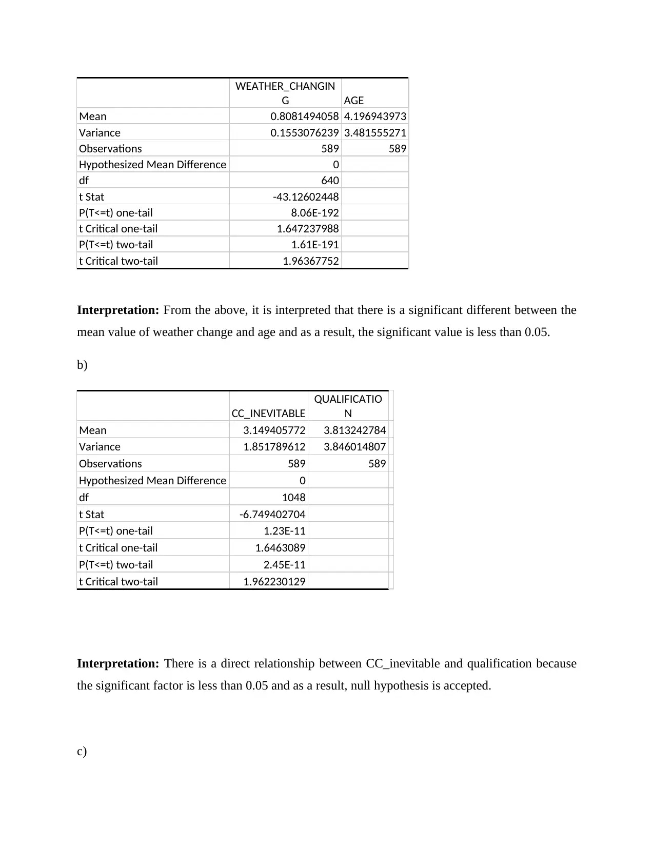
WEATHER_CHANGIN
G AGE
Mean 0.8081494058 4.196943973
Variance 0.1553076239 3.481555271
Observations 589 589
Hypothesized Mean Difference 0
df 640
t Stat -43.12602448
P(T<=t) one-tail 8.06E-192
t Critical one-tail 1.647237988
P(T<=t) two-tail 1.61E-191
t Critical two-tail 1.96367752
Interpretation: From the above, it is interpreted that there is a significant different between the
mean value of weather change and age and as a result, the significant value is less than 0.05.
b)
CC_INEVITABLE
QUALIFICATIO
N
Mean 3.149405772 3.813242784
Variance 1.851789612 3.846014807
Observations 589 589
Hypothesized Mean Difference 0
df 1048
t Stat -6.749402704
P(T<=t) one-tail 1.23E-11
t Critical one-tail 1.6463089
P(T<=t) two-tail 2.45E-11
t Critical two-tail 1.962230129
Interpretation: There is a direct relationship between CC_inevitable and qualification because
the significant factor is less than 0.05 and as a result, null hypothesis is accepted.
c)

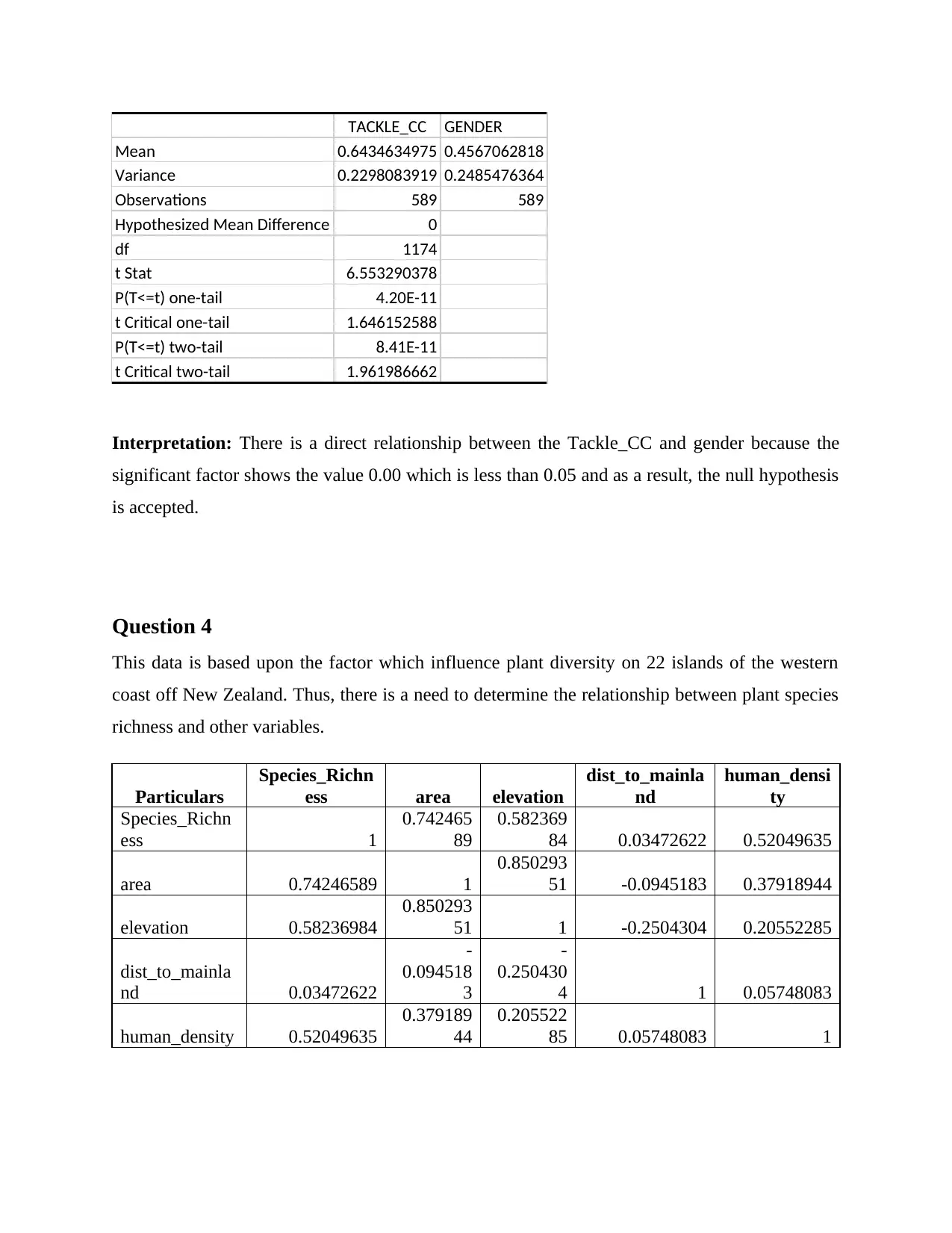
TACKLE_CC GENDER
Mean 0.6434634975 0.4567062818
Variance 0.2298083919 0.2485476364
Observations 589 589
Hypothesized Mean Difference 0
df 1174
t Stat 6.553290378
P(T<=t) one-tail 4.20E-11
t Critical one-tail 1.646152588
P(T<=t) two-tail 8.41E-11
t Critical two-tail 1.961986662
Interpretation: There is a direct relationship between the Tackle_CC and gender because the
significant factor shows the value 0.00 which is less than 0.05 and as a result, the null hypothesis
is accepted.
Question 4
This data is based upon the factor which influence plant diversity on 22 islands of the western
coast off New Zealand. Thus, there is a need to determine the relationship between plant species
richness and other variables.
Particulars
Species_Richn
ess area elevation
dist_to_mainla
nd
human_densi
ty
Species_Richn
ess 1
0.742465
89
0.582369
84 0.03472622 0.52049635
area 0.74246589 1
0.850293
51 -0.0945183 0.37918944
elevation 0.58236984
0.850293
51 1 -0.2504304 0.20552285
dist_to_mainla
nd 0.03472622
-
0.094518
3
-
0.250430
4 1 0.05748083
human_density 0.52049635
0.379189
44
0.205522
85 0.05748083 1

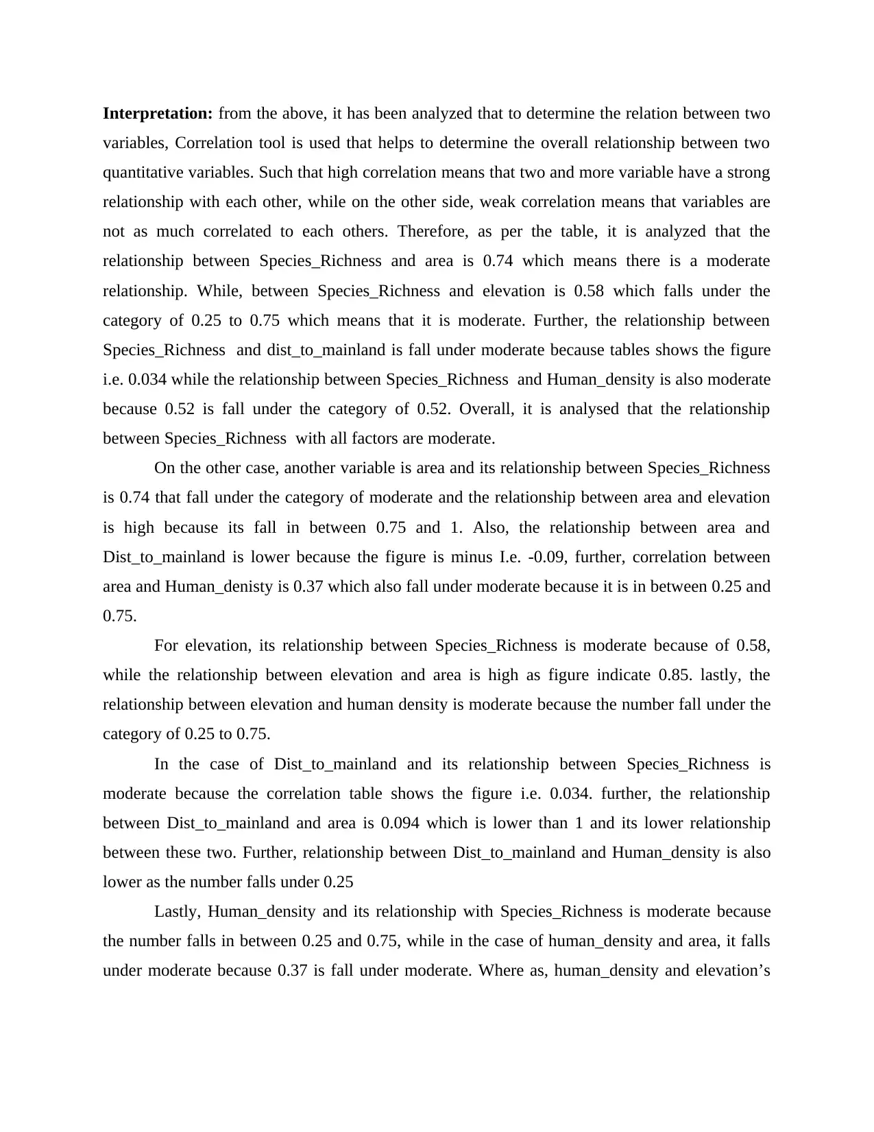
Interpretation: from the above, it has been analyzed that to determine the relation between two
variables, Correlation tool is used that helps to determine the overall relationship between two
quantitative variables. Such that high correlation means that two and more variable have a strong
relationship with each other, while on the other side, weak correlation means that variables are
not as much correlated to each others. Therefore, as per the table, it is analyzed that the
relationship between Species_Richness and area is 0.74 which means there is a moderate
relationship. While, between Species_Richness and elevation is 0.58 which falls under the
category of 0.25 to 0.75 which means that it is moderate. Further, the relationship between
Species_Richness and dist_to_mainland is fall under moderate because tables shows the figure
i.e. 0.034 while the relationship between Species_Richness and Human_density is also moderate
because 0.52 is fall under the category of 0.52. Overall, it is analysed that the relationship
between Species_Richness with all factors are moderate.
On the other case, another variable is area and its relationship between Species_Richness
is 0.74 that fall under the category of moderate and the relationship between area and elevation
is high because its fall in between 0.75 and 1. Also, the relationship between area and
Dist_to_mainland is lower because the figure is minus I.e. -0.09, further, correlation between
area and Human_denisty is 0.37 which also fall under moderate because it is in between 0.25 and
0.75.
For elevation, its relationship between Species_Richness is moderate because of 0.58,
while the relationship between elevation and area is high as figure indicate 0.85. lastly, the
relationship between elevation and human density is moderate because the number fall under the
category of 0.25 to 0.75.
In the case of Dist_to_mainland and its relationship between Species_Richness is
moderate because the correlation table shows the figure i.e. 0.034. further, the relationship
between Dist_to_mainland and area is 0.094 which is lower than 1 and its lower relationship
between these two. Further, relationship between Dist_to_mainland and Human_density is also
lower as the number falls under 0.25
Lastly, Human_density and its relationship with Species_Richness is moderate because
the number falls in between 0.25 and 0.75, while in the case of human_density and area, it falls
under moderate because 0.37 is fall under moderate. Where as, human_density and elevation’s

relation is lower because it fall under the category of 0.1 to 0.25, on the other hand, the variable
relationship with its own is 1 that is also indicate high relationship in all the cases.