Data Analysis Techniques

This report provides an understanding of data analysis techniques, including representation of data in tabular form and charts, calculations of mean, median, mode, standard deviation, and range. It also explains the use of linear forecasting model for predicting future values.

Data analysis techniques

Contents
INTRODUCTION...........................................................................................................................1
MAIN BODY..................................................................................................................................1
Representation of data in tabular form........................................................................................1
Data representation in charts.......................................................................................................2
Calculations of mean, median, mode, standard deviation and range...........................................2
Calculating values of m, c and gas bill of Month 12 and 14.......................................................4
CONCLUSION................................................................................................................................6
REFERENCES................................................................................................................................7

INTRODUCTION
Data analysis is the technique of recording, classifying and analysing the data for the
purpose of viable decision making. This concept is related the data which can be further used for
predicting future variables (Landtblom, 2018). The main aim of this report is build an
understanding about the process of analysing a data using statistical measures. In this report, 10
Months data of gas bill is acquired and then recoded using tables and graphs. This data is
evaluated using descriptive analysis techniques of Mean, mode, median, range and standard
deviation. Lastly, this data is used to predict Month 12 and 14th gas bill using linear forecasting
technique.
MAIN BODY
Representation of data in tabular form
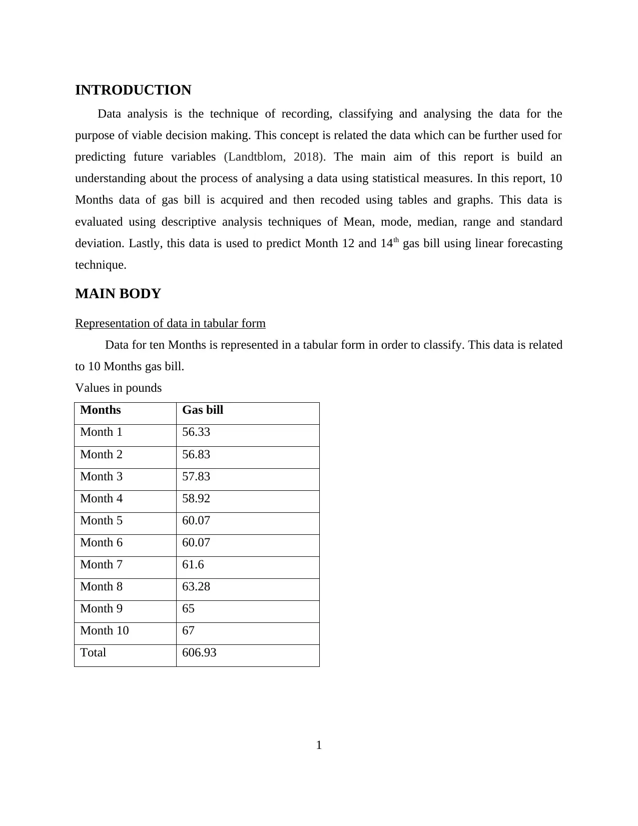
Data for ten Months is represented in a tabular form in order to classify. This data is related
to 10 Months gas bill.
Values in pounds
Months Gas bill
Month 1 56.33
Month 2 56.83
Month 3 57.83
Month 4 58.92
Month 5 60.07
Month 6 60.07
Month 7 61.6
Month 8 63.28
Month 9 65
Month 10 67
Total 606.93
1

Data representation in charts
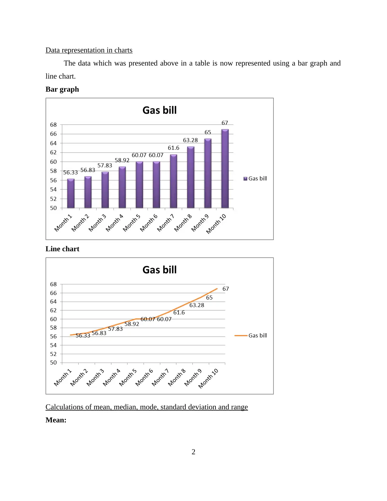
The data which was presented above in a table is now represented using a bar graph and
line chart.
Bar graph
Line chart
Calculations of mean, median, mode, standard deviation and range
Mean:
2

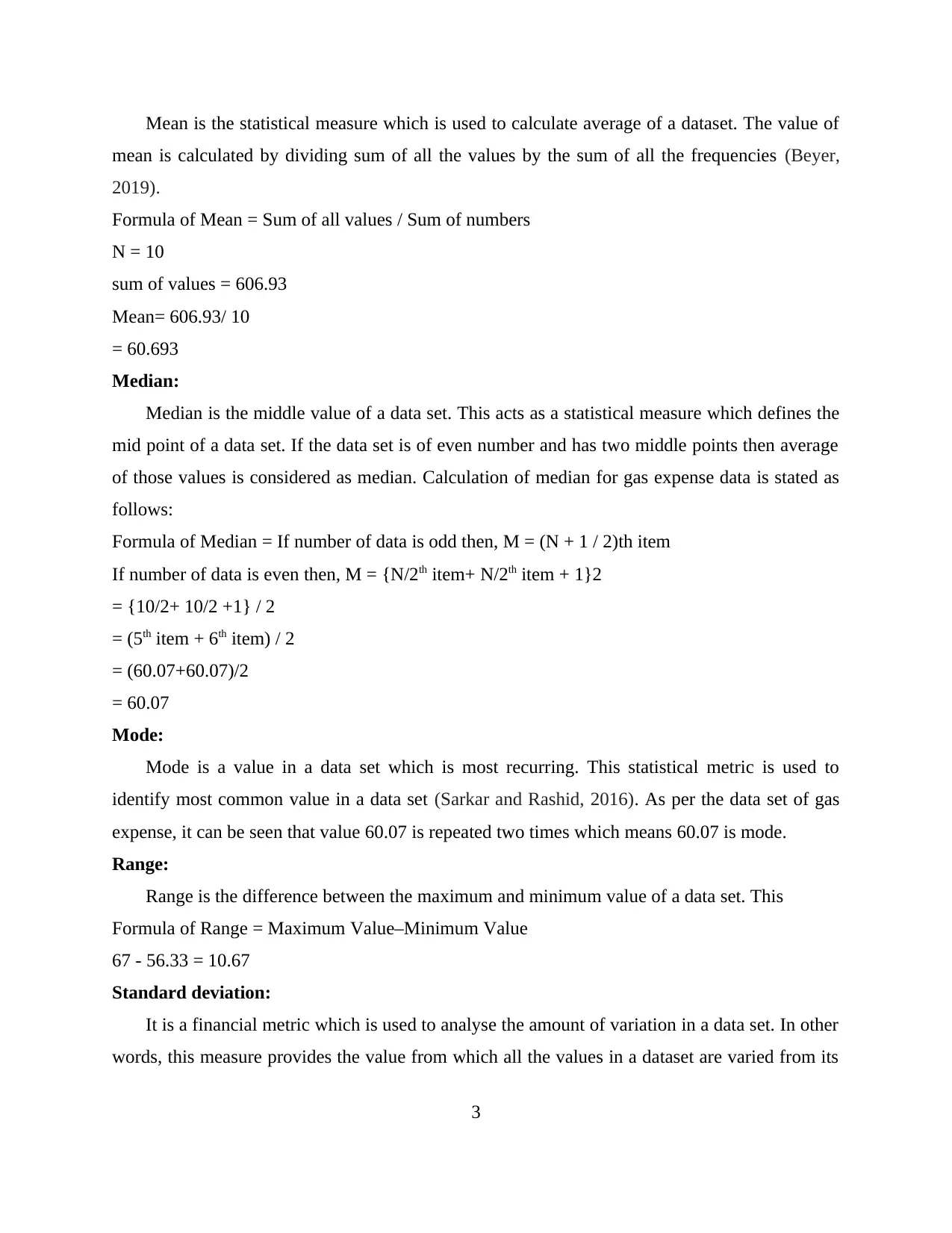
Mean is the statistical measure which is used to calculate average of a dataset. The value of
mean is calculated by dividing sum of all the values by the sum of all the frequencies (Beyer,
2019).
Formula of Mean = Sum of all values / Sum of numbers
N = 10
sum of values = 606.93
Mean= 606.93/ 10
= 60.693
Median:
Median is the middle value of a data set. This acts as a statistical measure which defines the
mid point of a data set. If the data set is of even number and has two middle points then average
of those values is considered as median. Calculation of median for gas expense data is stated as
follows:
Formula of Median = If number of data is odd then, M = (N + 1 / 2)th item
If number of data is even then, M = {N/2th item+ N/2th item + 1}2
= {10/2+ 10/2 +1} / 2
= (5th item + 6th item) / 2
= (60.07+60.07)/2
= 60.07
Mode:
Mode is a value in a data set which is most recurring. This statistical metric is used to
identify most common value in a data set (Sarkar and Rashid, 2016). As per the data set of gas
expense, it can be seen that value 60.07 is repeated two times which means 60.07 is mode.
Range:
Range is the difference between the maximum and minimum value of a data set. This
Formula of Range = Maximum Value–Minimum Value
67 - 56.33 = 10.67
Standard deviation:
It is a financial metric which is used to analyse the amount of variation in a data set. In other
words, this measure provides the value from which all the values in a dataset are varied from its
3

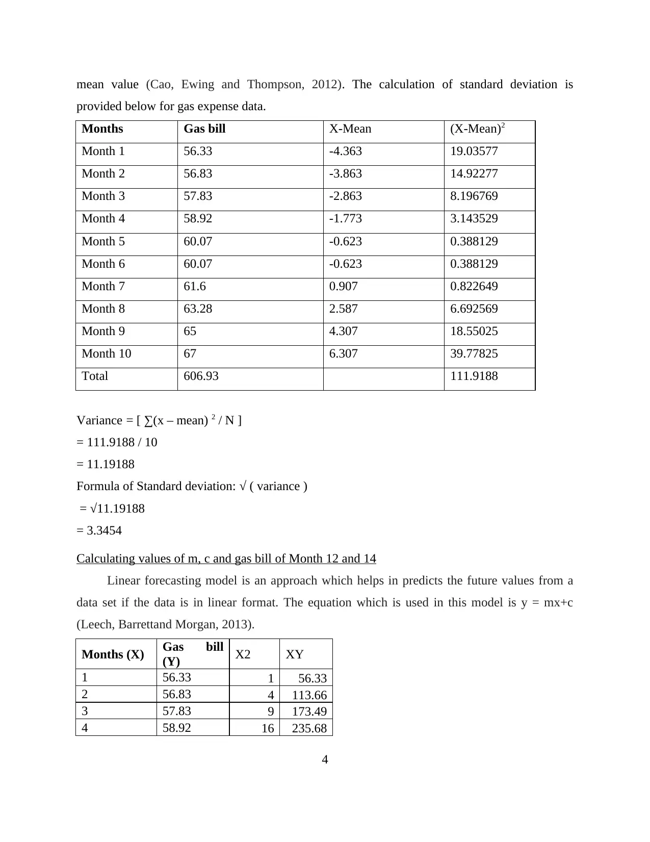
mean value (Cao, Ewing and Thompson, 2012). The calculation of standard deviation is
provided below for gas expense data.
Months Gas bill X-Mean (X-Mean)2
Month 1 56.33 -4.363 19.03577
Month 2 56.83 -3.863 14.92277
Month 3 57.83 -2.863 8.196769
Month 4 58.92 -1.773 3.143529
Month 5 60.07 -0.623 0.388129
Month 6 60.07 -0.623 0.388129
Month 7 61.6 0.907 0.822649
Month 8 63.28 2.587 6.692569
Month 9 65 4.307 18.55025
Month 10 67 6.307 39.77825
Total 606.93 111.9188
Variance = [ ∑(x – mean) 2 / N ]
= 111.9188 / 10
= 11.19188
Formula of Standard deviation: √ ( variance )
= √11.19188
= 3.3454
Calculating values of m, c and gas bill of Month 12 and 14
Linear forecasting model is an approach which helps in predicts the future values from a
data set if the data is in linear format. The equation which is used in this model is y = mx+c
(Leech, Barrettand Morgan, 2013).
Months (X) Gas bill
(Y) X2 XY
1 56.33 1 56.33
2 56.83 4 113.66
3 57.83 9 173.49
4 58.92 16 235.68
4

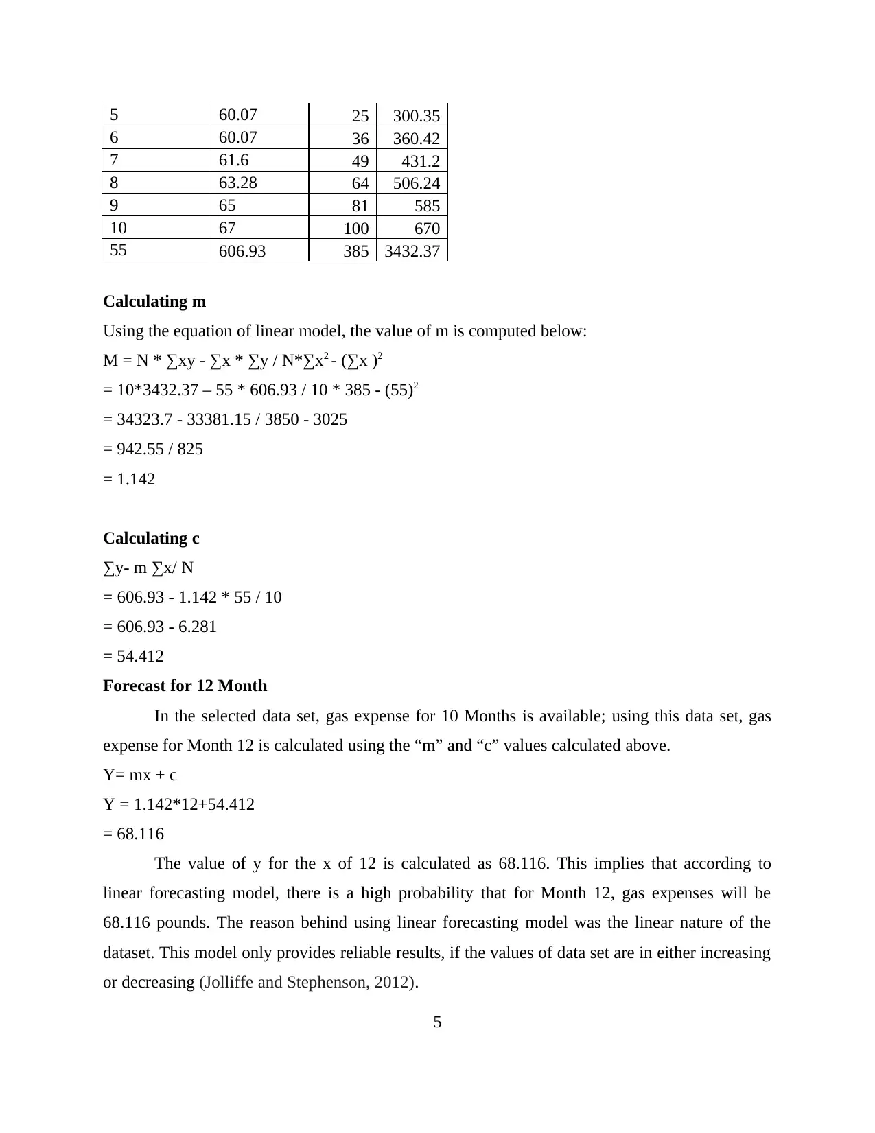
5 60.07 25 300.35
6 60.07 36 360.42
7 61.6 49 431.2
8 63.28 64 506.24
9 65 81 585
10 67 100 670
55 606.93 385 3432.37
Calculating m
Using the equation of linear model, the value of m is computed below:
M = N * ∑xy - ∑x * ∑y / N*∑x2 - (∑x )2
= 10*3432.37 – 55 * 606.93 / 10 * 385 - (55)2
= 34323.7 - 33381.15 / 3850 - 3025
= 942.55 / 825
= 1.142
Calculating c
∑y- m ∑x/ N
= 606.93 - 1.142 * 55 / 10
= 606.93 - 6.281
= 54.412
Forecast for 12 Month
In the selected data set, gas expense for 10 Months is available; using this data set, gas
expense for Month 12 is calculated using the “m” and “c” values calculated above.
Y= mx + c
Y = 1.142*12+54.412
= 68.116
The value of y for the x of 12 is calculated as 68.116. This implies that according to
linear forecasting model, there is a high probability that for Month 12, gas expenses will be
68.116 pounds. The reason behind using linear forecasting model was the linear nature of the
dataset. This model only provides reliable results, if the values of data set are in either increasing
or decreasing (Jolliffe and Stephenson, 2012).
5

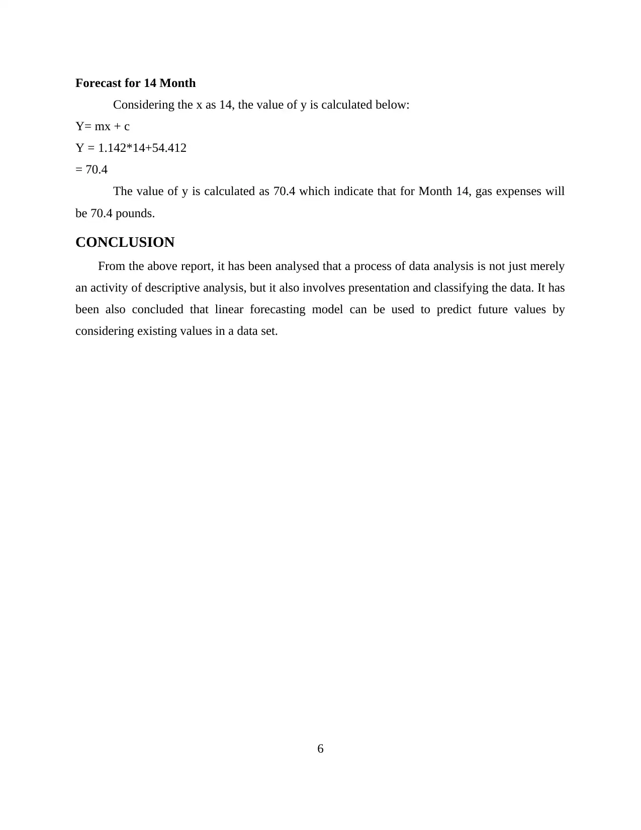
Forecast for 14 Month
Considering the x as 14, the value of y is calculated below:
Y= mx + c
Y = 1.142*14+54.412
= 70.4
The value of y is calculated as 70.4 which indicate that for Month 14, gas expenses will
be 70.4 pounds.
CONCLUSION
From the above report, it has been analysed that a process of data analysis is not just merely
an activity of descriptive analysis, but it also involves presentation and classifying the data. It has
been also concluded that linear forecasting model can be used to predict future values by
considering existing values in a data set.
6

REFERENCES
Books and Journals
Beyer, W. H., 2019. Handbook of tables for probability and statistics. Crc Press.
Cao, Q., Ewing, B.T. and Thompson, M.A., 2012. Forecasting wind speed with recurrent neural
networks. European Journal of Operational Research. 221(1). pp.148-154.
Jolliffe, I.T. and Stephenson, D.B. eds., 2012. Forecast verification: a practitioner's guide in
atmospheric science. John Wiley & Sons.
Landtblom, K. K., 2018. Prospective Teachers’ Conceptions of the Concepts Mean, Median and
Mode. In Students' and Teachers' Values, Attitudes, Feelings and Beliefs in
Mathematics Classrooms (pp. 43-52). Springer, Cham.
Leech, N., Barrett, K. and Morgan, G. A., 2013. SPSS for intermediate statistics: Use and
interpretation. Routledge.
Sarkar, J. and Rashid, M., 2016. Visualizing mean, median, mean deviation, and standard
deviation of a set of numbers. The American Statistician. 70(3). pp.304-312.
7