Data Analytics: A Business Case Study

Data Analytics: A Business Case Study from online shopping
Executive Summary
Today most of the world population preferred the online shopping which results into
the exponential growth in eCommerce. eCommerce becoming very raising and popular
business in every corner of the world. Online shopping is most popular from the all
eCommerce business. In Today’s market we can see the words like Amazon, eBay, etc.
which very common in day to day life. Service provider attract the customer by giving offers
to the customers.
Growth in the online shopping creates the opportunity and challenges to the service
provider. The main challenges in the online shopping is competition and customer total
satisfaction.
We have data sets regarding to Cloths (Shirt, Trouser and Track Suit) for the 2000
products. We summarised the total sale amount and total profit in profit analysis. We carried
the chi-squared test for association of attributes (shipping type, customer type, region, brand
and material). We analyzed the mean of number of customers for shipping type, customer
type, region, brand and material by the two sample t test and one way ANOVA. We also
carried correlation analysis. Recommendation and plan is also provided from the analysis.
1

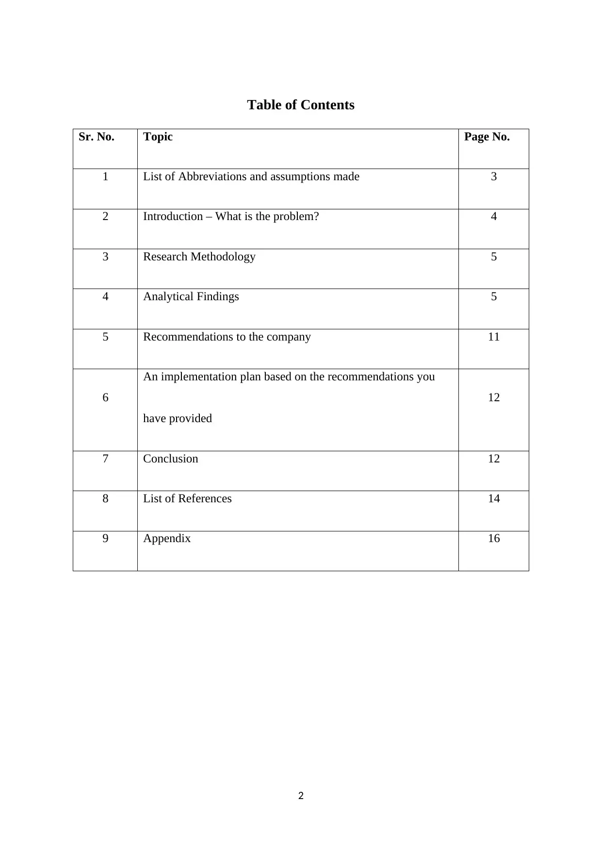
Table of Contents
Sr. No. Topic Page No.
1 List of Abbreviations and assumptions made 3
2 Introduction – What is the problem? 4
3 Research Methodology 5
4 Analytical Findings 5
5 Recommendations to the company 11
6
An implementation plan based on the recommendations you
have provided
12
7 Conclusion 12
8 List of References 14
9 Appendix 16
2

List of Abbreviations and assumptions made
Max : Maximum
Min : Minimum
QLD : Queensland
TAS : Tasmania
VIC : Victoria
WA : Western Australia
3

Introduction – What is the problem?
Today most of the world population preferred the online shopping which results into
the exponential growth in eCommerce. eCommerce becoming very raising and popular
business in every corner of the world. Online shopping is most popular from the all
eCommerce business. In Today’s market we can see the words like Amazon, eBay, etc.
which very common in day to day life. Service provider attract the customer by giving offers
to the customers.
Growth in the online shopping creates the opportunity and challenges to the service
provider. The main challenges in the online shopping is competition and customer total
satisfaction.
About Data:
We have data sets regarding to Cloths (Shirt, Trouser and Track Suit) for the 2000
products. We considered the following attributes
i) Product Name
ii) Product Price (in $)
iii) Sale Price (in $)
iv) Profit (in $)
v) Number of customers
vi) Shipping Type (Free or Paid)
vii) Customer Type (New or Existing)
viii) Region (QLD, WA, VIC, TAS)
ix) Product Brand
x) Product Material
We define following variables for our analysis from the above variables
4

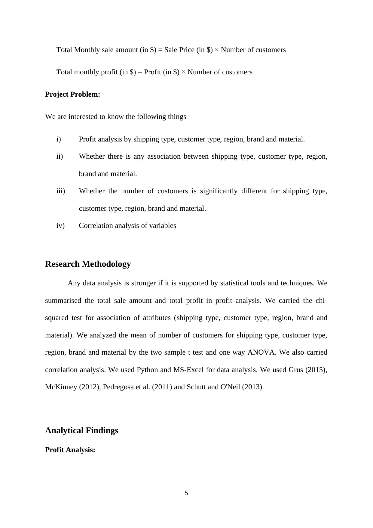
Total Monthly sale amount (in $) = Sale Price (in $) × Number of customers
Total monthly profit (in $) = Profit (in $) × Number of customers
Project Problem:
We are interested to know the following things
i) Profit analysis by shipping type, customer type, region, brand and material.
ii) Whether there is any association between shipping type, customer type, region,
brand and material.
iii) Whether the number of customers is significantly different for shipping type,
customer type, region, brand and material.
iv) Correlation analysis of variables
Research Methodology
Any data analysis is stronger if it is supported by statistical tools and techniques. We
summarised the total sale amount and total profit in profit analysis. We carried the chi-
squared test for association of attributes (shipping type, customer type, region, brand and
material). We analyzed the mean of number of customers for shipping type, customer type,
region, brand and material by the two sample t test and one way ANOVA. We also carried
correlation analysis. We used Python and MS-Excel for data analysis. We used Grus (2015),
McKinney (2012), Pedregosa et al. (2011) and Schutt and O'Neil (2013).
Analytical Findings
Profit Analysis:
5

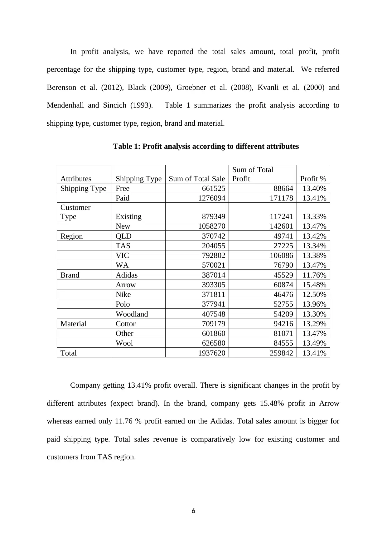
In profit analysis, we have reported the total sales amount, total profit, profit
percentage for the shipping type, customer type, region, brand and material. We referred
Berenson et al. (2012), Black (2009), Groebner et al. (2008), Kvanli et al. (2000) and
Mendenhall and Sincich (1993). Table 1 summarizes the profit analysis according to
shipping type, customer type, region, brand and material.
Table 1: Profit analysis according to different attributes
Attributes Shipping Type Sum of Total Sale
Sum of Total
Profit Profit %
Shipping Type Free 661525 88664 13.40%
Paid 1276094 171178 13.41%
Customer
Type Existing 879349 117241 13.33%
New 1058270 142601 13.47%
Region QLD 370742 49741 13.42%
TAS 204055 27225 13.34%
VIC 792802 106086 13.38%
WA 570021 76790 13.47%
Brand Adidas 387014 45529 11.76%
Arrow 393305 60874 15.48%
Nike 371811 46476 12.50%
Polo 377941 52755 13.96%
Woodland 407548 54209 13.30%
Material Cotton 709179 94216 13.29%
Other 601860 81071 13.47%
Wool 626580 84555 13.49%
Total 1937620 259842 13.41%
Company getting 13.41% profit overall. There is significant changes in the profit by
different attributes (expect brand). In the brand, company gets 15.48% profit in Arrow
whereas earned only 11.76 % profit earned on the Adidas. Total sales amount is bigger for
paid shipping type. Total sales revenue is comparatively low for existing customer and
customers from TAS region.
6

Descriptive statistics:
We used the well-known books for this section such as Bickel and Doksum (2015),
Casella and Berger (2002), DeGroot and Schervish (2012), Hodges Jr and Lehmann (2005),
Papoulis (1990), Pillers (2002) and Ross (2014).
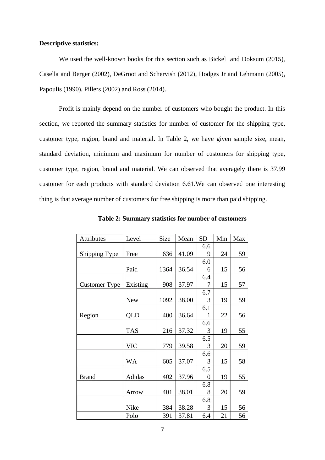
Profit is mainly depend on the number of customers who bought the product. In this
section, we reported the summary statistics for number of customer for the shipping type,
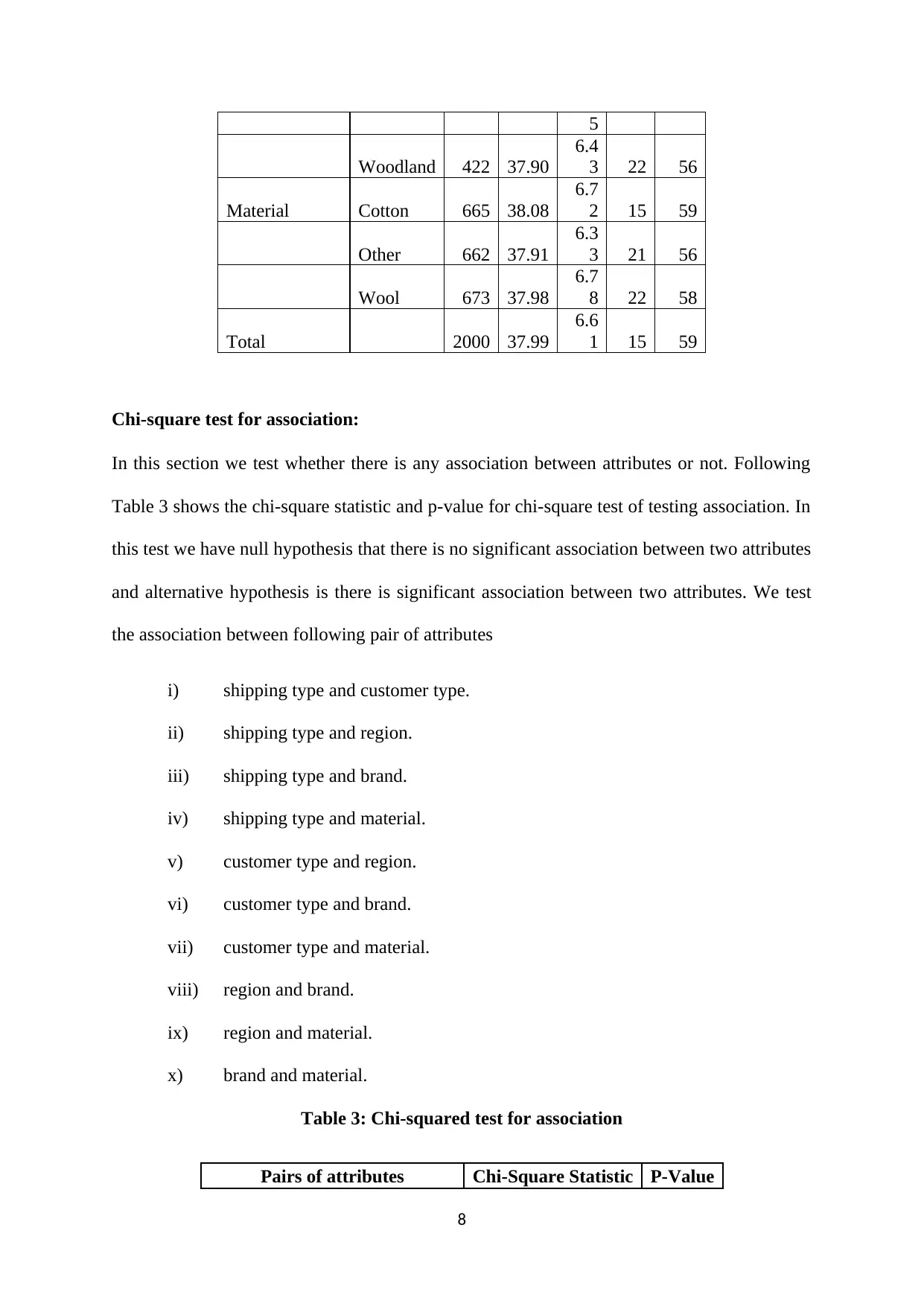
customer type, region, brand and material. In Table 2, we have given sample size, mean,
standard deviation, minimum and maximum for number of customers for shipping type,
customer type, region, brand and material. We can observed that averagely there is 37.99
customer for each products with standard deviation 6.61.We can observed one interesting
thing is that average number of customers for free shipping is more than paid shipping.
Table 2: Summary statistics for number of customers
Attributes Level Size Mean SD Min Max
Shipping Type Free 636 41.09
6.6
9 24 59
Paid 1364 36.54
6.0
6 15 56
Customer Type Existing 908 37.97
6.4
7 15 57
New 1092 38.00
6.7
3 19 59
Region QLD 400 36.64
6.1
1 22 56
TAS 216 37.32
6.6
3 19 55
VIC 779 39.58
6.5
3 20 59
WA 605 37.07
6.6
3 15 58
Brand Adidas 402 37.96
6.5
0 19 55
Arrow 401 38.01
6.8
8 20 59
Nike 384 38.28
6.8
3 15 56
Polo 391 37.81 6.4 21 56
7

5
Woodland 422 37.90
6.4
3 22 56
Material Cotton 665 38.08
6.7
2 15 59
Other 662 37.91
6.3
3 21 56
Wool 673 37.98
6.7
8 22 58
Total 2000 37.99
6.6
1 15 59
Chi-square test for association:
In this section we test whether there is any association between attributes or not. Following
Table 3 shows the chi-square statistic and p-value for chi-square test of testing association. In
this test we have null hypothesis that there is no significant association between two attributes
and alternative hypothesis is there is significant association between two attributes. We test
the association between following pair of attributes
i) shipping type and customer type.
ii) shipping type and region.
iii) shipping type and brand.
iv) shipping type and material.
v) customer type and region.
vi) customer type and brand.
vii) customer type and material.
viii) region and brand.
ix) region and material.
x) brand and material.
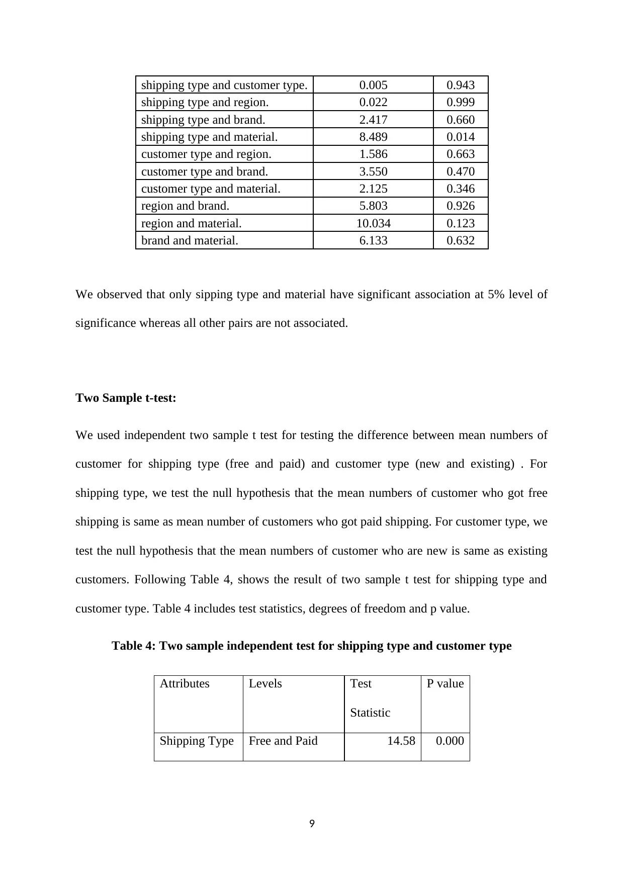
Table 3: Chi-squared test for association
Pairs of attributes Chi-Square Statistic P-Value
8

shipping type and customer type. 0.005 0.943
shipping type and region. 0.022 0.999
shipping type and brand. 2.417 0.660
shipping type and material. 8.489 0.014
customer type and region. 1.586 0.663
customer type and brand. 3.550 0.470
customer type and material. 2.125 0.346
region and brand. 5.803 0.926
region and material. 10.034 0.123
brand and material. 6.133 0.632
We observed that only sipping type and material have significant association at 5% level of
significance whereas all other pairs are not associated.
Two Sample t-test:
We used independent two sample t test for testing the difference between mean numbers of
customer for shipping type (free and paid) and customer type (new and existing) . For
shipping type, we test the null hypothesis that the mean numbers of customer who got free
shipping is same as mean number of customers who got paid shipping. For customer type, we
test the null hypothesis that the mean numbers of customer who are new is same as existing
customers. Following Table 4, shows the result of two sample t test for shipping type and
customer type. Table 4 includes test statistics, degrees of freedom and p value.
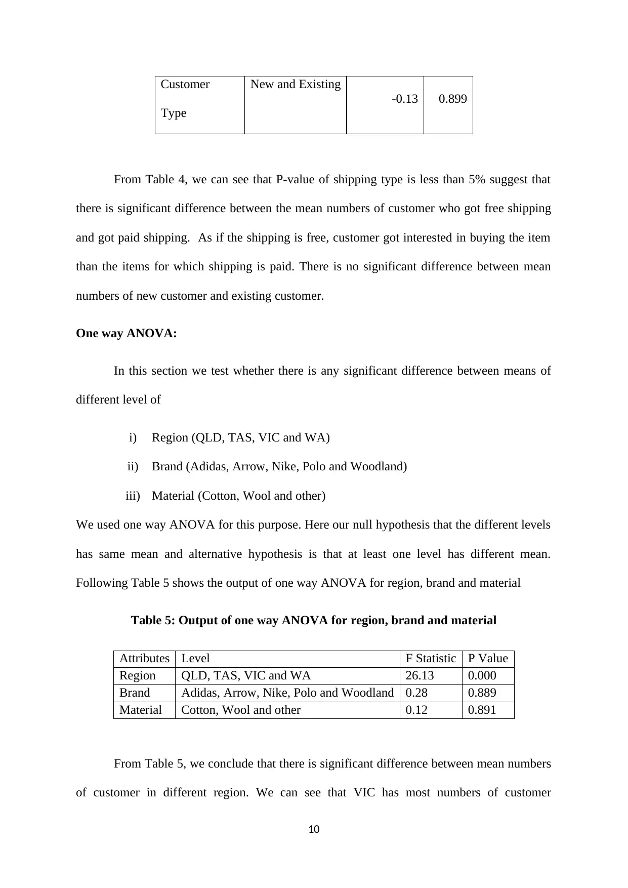
Table 4: Two sample independent test for shipping type and customer type
Attributes Levels Test
Statistic
P value
Shipping Type Free and Paid 14.58 0.000
9

Customer
Type
New and Existing
-0.13 0.899
From Table 4, we can see that P-value of shipping type is less than 5% suggest that
there is significant difference between the mean numbers of customer who got free shipping
and got paid shipping. As if the shipping is free, customer got interested in buying the item
than the items for which shipping is paid. There is no significant difference between mean
numbers of new customer and existing customer.
One way ANOVA:
In this section we test whether there is any significant difference between means of
different level of
i) Region (QLD, TAS, VIC and WA)
ii) Brand (Adidas, Arrow, Nike, Polo and Woodland)
iii) Material (Cotton, Wool and other)
We used one way ANOVA for this purpose. Here our null hypothesis that the different levels
has same mean and alternative hypothesis is that at least one level has different mean.
Following Table 5 shows the output of one way ANOVA for region, brand and material
Table 5: Output of one way ANOVA for region, brand and material
Attributes Level F Statistic P Value
Region QLD, TAS, VIC and WA 26.13 0.000
Brand Adidas, Arrow, Nike, Polo and Woodland 0.28 0.889
Material Cotton, Wool and other 0.12 0.891
From Table 5, we conclude that there is significant difference between mean numbers
of customer in different region. We can see that VIC has most numbers of customer
10

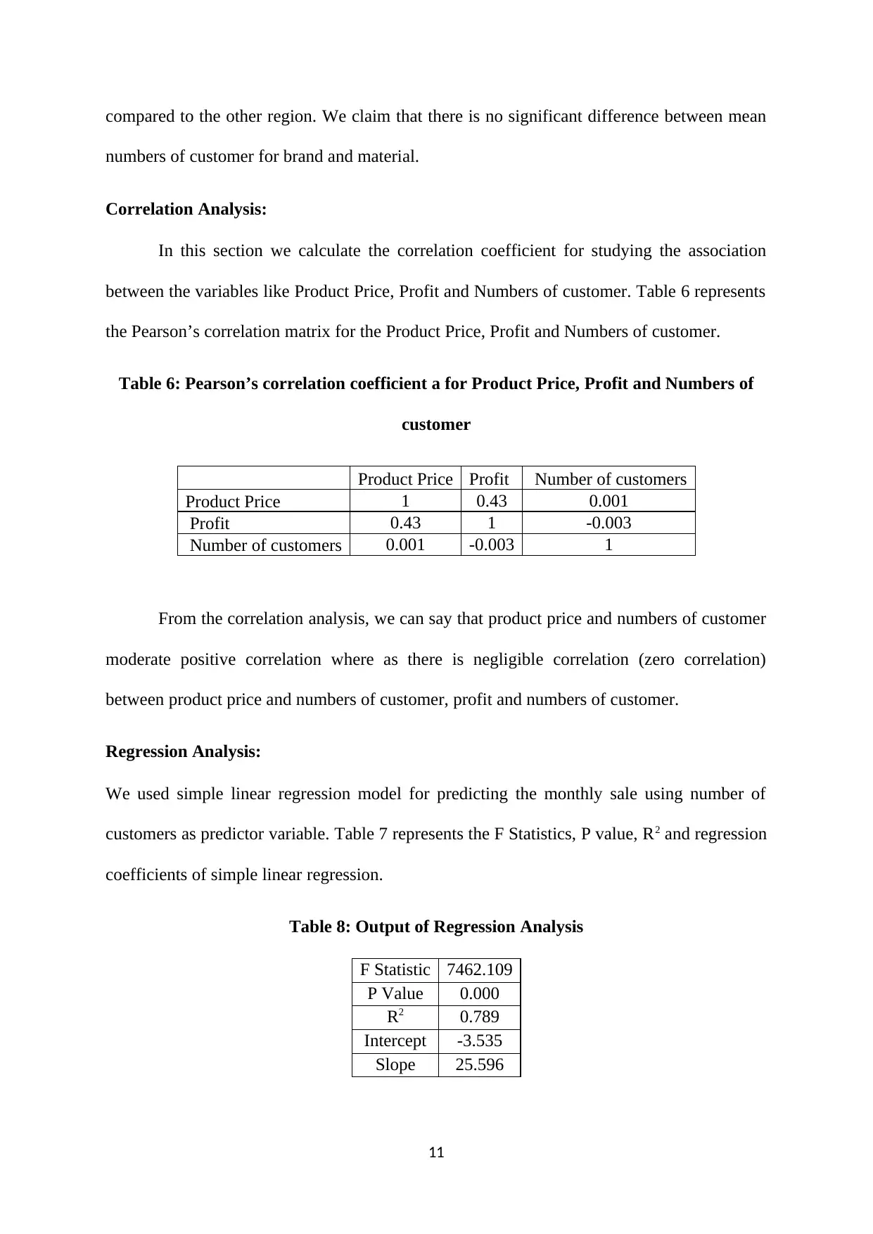
compared to the other region. We claim that there is no significant difference between mean
numbers of customer for brand and material.
Correlation Analysis:
In this section we calculate the correlation coefficient for studying the association
between the variables like Product Price, Profit and Numbers of customer. Table 6 represents
the Pearson’s correlation matrix for the Product Price, Profit and Numbers of customer.
Table 6: Pearson’s correlation coefficient a for Product Price, Profit and Numbers of
customer
Product Price Profit Number of customers
Product Price 1 0.43 0.001
Profit 0.43 1 -0.003
Number of customers 0.001 -0.003 1
From the correlation analysis, we can say that product price and numbers of customer
moderate positive correlation where as there is negligible correlation (zero correlation)
between product price and numbers of customer, profit and numbers of customer.
Regression Analysis:
We used simple linear regression model for predicting the monthly sale using number of
customers as predictor variable. Table 7 represents the F Statistics, P value, R2 and regression
coefficients of simple linear regression.
Table 8: Output of Regression Analysis
F Statistic 7462.109
P Value 0.000
R2 0.789
Intercept -3.535
Slope 25.596
11

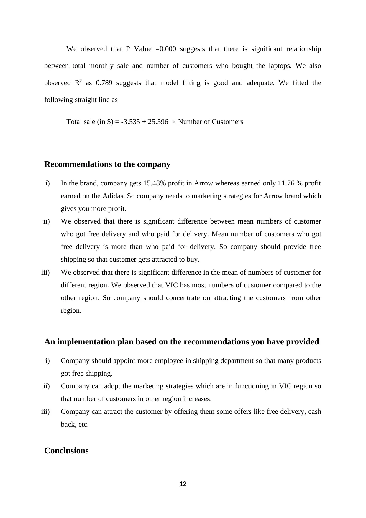
We observed that P Value =0.000 suggests that there is significant relationship
between total monthly sale and number of customers who bought the laptops. We also
observed R2 as 0.789 suggests that model fitting is good and adequate. We fitted the
following straight line as
Total sale (in $) = -3.535 + 25.596 × Number of Customers
Recommendations to the company
i) In the brand, company gets 15.48% profit in Arrow whereas earned only 11.76 % profit
earned on the Adidas. So company needs to marketing strategies for Arrow brand which
gives you more profit.
ii) We observed that there is significant difference between mean numbers of customer
who got free delivery and who paid for delivery. Mean number of customers who got
free delivery is more than who paid for delivery. So company should provide free
shipping so that customer gets attracted to buy.
iii) We observed that there is significant difference in the mean of numbers of customer for
different region. We observed that VIC has most numbers of customer compared to the
other region. So company should concentrate on attracting the customers from other
region.
An implementation plan based on the recommendations you have provided
i) Company should appoint more employee in shipping department so that many products
got free shipping.
ii) Company can adopt the marketing strategies which are in functioning in VIC region so
that number of customers in other region increases.
iii) Company can attract the customer by offering them some offers like free delivery, cash
back, etc.
Conclusions
12

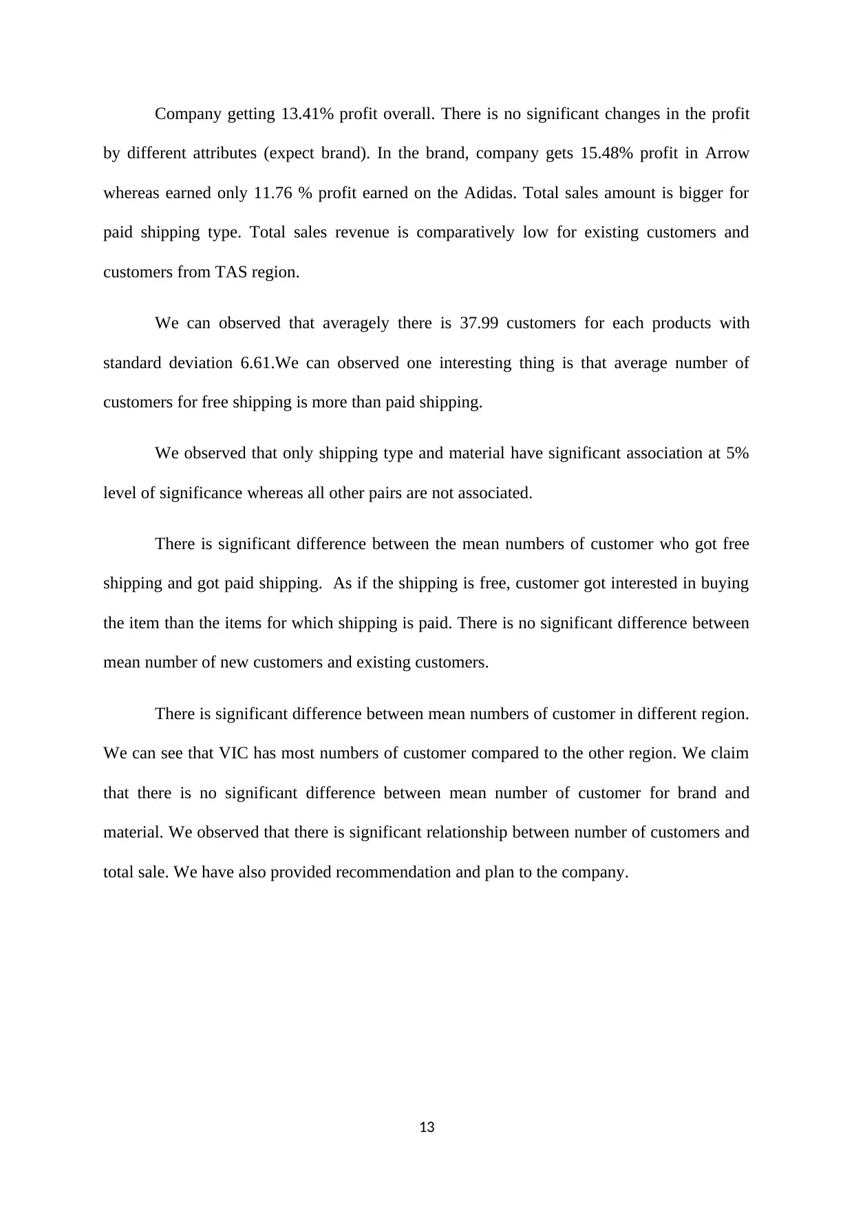
Company getting 13.41% profit overall. There is no significant changes in the profit
by different attributes (expect brand). In the brand, company gets 15.48% profit in Arrow
whereas earned only 11.76 % profit earned on the Adidas. Total sales amount is bigger for
paid shipping type. Total sales revenue is comparatively low for existing customers and
customers from TAS region.
We can observed that averagely there is 37.99 customers for each products with
standard deviation 6.61.We can observed one interesting thing is that average number of
customers for free shipping is more than paid shipping.
We observed that only shipping type and material have significant association at 5%
level of significance whereas all other pairs are not associated.
There is significant difference between the mean numbers of customer who got free
shipping and got paid shipping. As if the shipping is free, customer got interested in buying
the item than the items for which shipping is paid. There is no significant difference between
mean number of new customers and existing customers.
There is significant difference between mean numbers of customer in different region.
We can see that VIC has most numbers of customer compared to the other region. We claim
that there is no significant difference between mean number of customer for brand and
material. We observed that there is significant relationship between number of customers and
total sale. We have also provided recommendation and plan to the company.
13

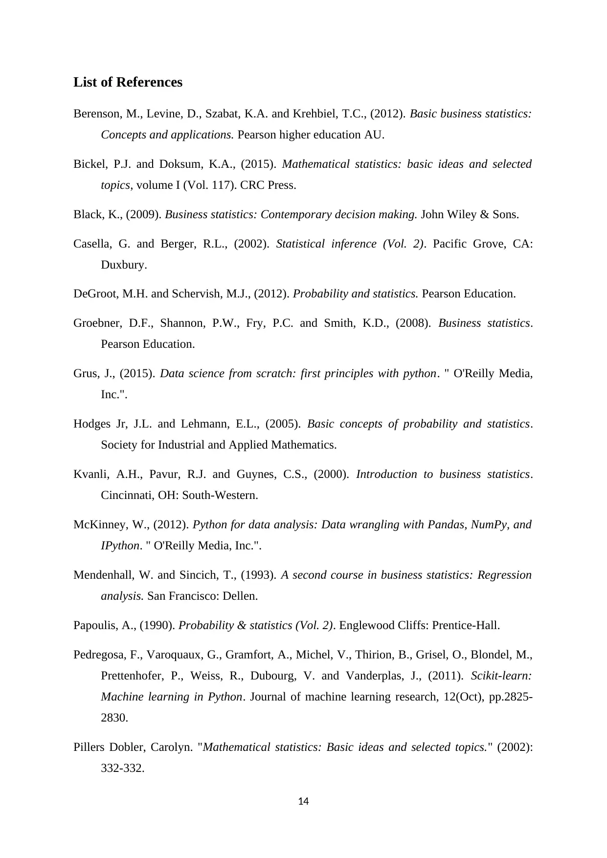
List of References
Berenson, M., Levine, D., Szabat, K.A. and Krehbiel, T.C., (2012). Basic business statistics:
Concepts and applications. Pearson higher education AU.
Bickel, P.J. and Doksum, K.A., (2015). Mathematical statistics: basic ideas and selected
topics, volume I (Vol. 117). CRC Press.
Black, K., (2009). Business statistics: Contemporary decision making. John Wiley & Sons.
Casella, G. and Berger, R.L., (2002). Statistical inference (Vol. 2). Pacific Grove, CA:
Duxbury.
DeGroot, M.H. and Schervish, M.J., (2012). Probability and statistics. Pearson Education.
Groebner, D.F., Shannon, P.W., Fry, P.C. and Smith, K.D., (2008). Business statistics.
Pearson Education.
Grus, J., (2015). Data science from scratch: first principles with python. " O'Reilly Media,
Inc.".
Hodges Jr, J.L. and Lehmann, E.L., (2005). Basic concepts of probability and statistics.
Society for Industrial and Applied Mathematics.
Kvanli, A.H., Pavur, R.J. and Guynes, C.S., (2000). Introduction to business statistics.
Cincinnati, OH: South-Western.
McKinney, W., (2012). Python for data analysis: Data wrangling with Pandas, NumPy, and
IPython. " O'Reilly Media, Inc.".
Mendenhall, W. and Sincich, T., (1993). A second course in business statistics: Regression
analysis. San Francisco: Dellen.
Papoulis, A., (1990). Probability & statistics (Vol. 2). Englewood Cliffs: Prentice-Hall.
Pedregosa, F., Varoquaux, G., Gramfort, A., Michel, V., Thirion, B., Grisel, O., Blondel, M.,
Prettenhofer, P., Weiss, R., Dubourg, V. and Vanderplas, J., (2011). Scikit-learn:
Machine learning in Python. Journal of machine learning research, 12(Oct), pp.2825-
2830.
Pillers Dobler, Carolyn. "Mathematical statistics: Basic ideas and selected topics." (2002):
332-332.
14

Ross, S.M., (2014). Introduction to probability and statistics for engineers and scientists.
Academic Press.
Schutt, R. and O'Neil, C., (2013). Doing data science: Straight talk from the frontline. "
O'Reilly Media, Inc.".
15

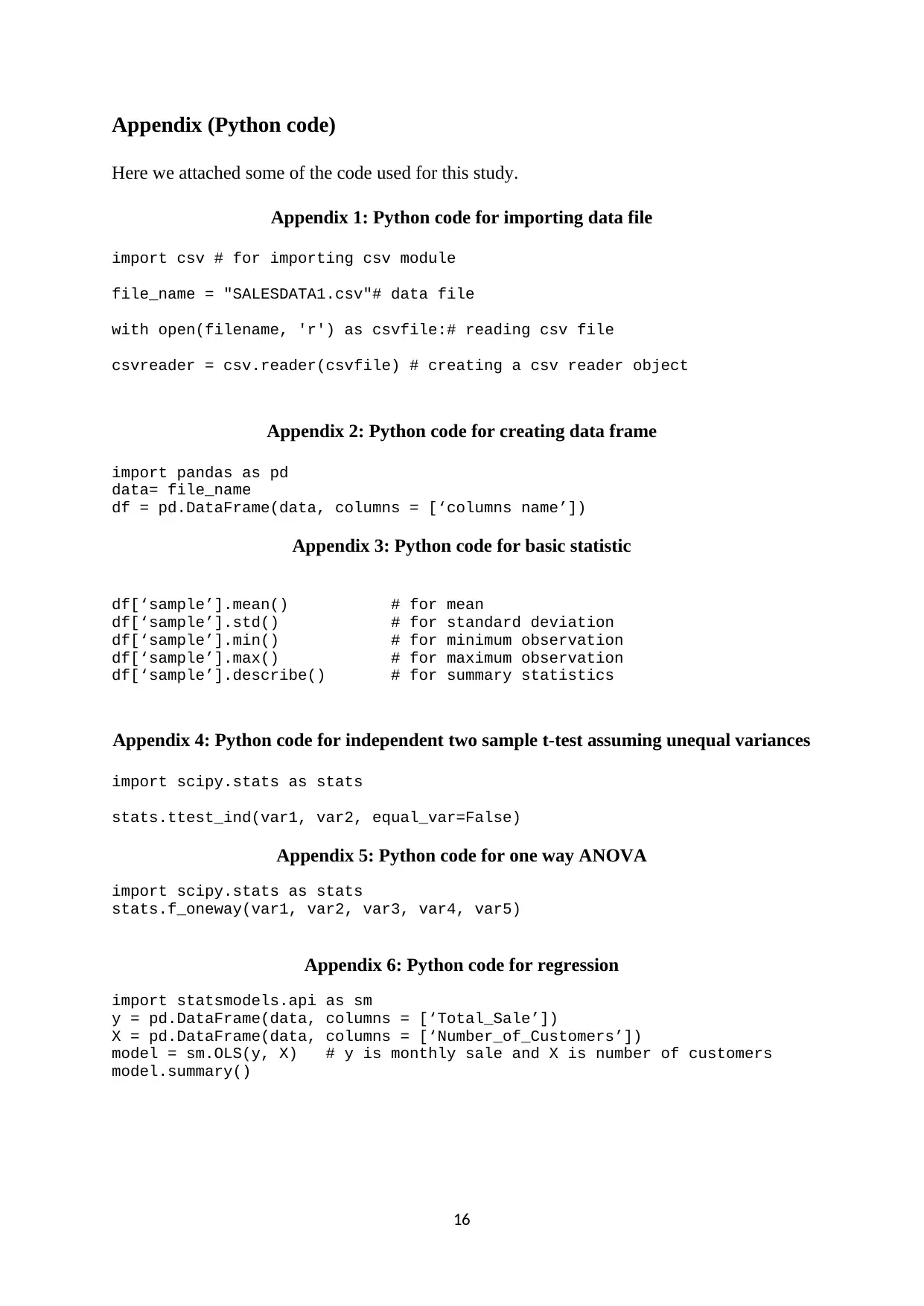
Appendix (Python code)
Here we attached some of the code used for this study.
Appendix 1: Python code for importing data file
import csv # for importing csv module
file_name = "SALESDATA1.csv"# data file
with open(filename, 'r') as csvfile:# reading csv file
csvreader = csv.reader(csvfile) # creating a csv reader object
Appendix 2: Python code for creating data frame
import pandas as pd
data= file_name
df = pd.DataFrame(data, columns = [‘columns name’])
Appendix 3: Python code for basic statistic
df[‘sample’].mean() # for mean
df[‘sample’].std() # for standard deviation
df[‘sample’].min() # for minimum observation
df[‘sample’].max() # for maximum observation
df[‘sample’].describe() # for summary statistics
Appendix 4: Python code for independent two sample t-test assuming unequal variances
import scipy.stats as stats
stats.ttest_ind(var1, var2, equal_var=False)
Appendix 5: Python code for one way ANOVA
import scipy.stats as stats
stats.f_oneway(var1, var2, var3, var4, var5)
Appendix 6: Python code for regression
import statsmodels.api as sm
y = pd.DataFrame(data, columns = [‘Total_Sale’])
X = pd.DataFrame(data, columns = [‘Number_of_Customers’])
model = sm.OLS(y, X) # y is monthly sale and X is number of customers
model.summary()
16