Business Intelligence and Data Analytics

This article discusses time series analysis, logistic regression, and forecasting methods in data analytics and business intelligence. It includes solved assignments and essays on these topics. The article also evaluates the output metrics and suggests the best prediction method. The cutoff value for odds and logit is explained, and the interpretation of total expenses-to-assets ratio in terms of the odds of being financially weak is provided. Finally, the article suggests adjusting the best cut-off value to reduce the cost of misclassification.

Running head: BUSINESS INTELLIGENCE AND DATA ANALYTICS
Business Intelligence and Data Analytics
Name
Course Number
Date
Faculty Name

DATA ANALYTICS AND BUSINESS INTELLIGENCE 2
Data Analytics and Business Intelligence
1. Time series analysis
a. Draw a scatterplot and interpret.
2013
2014
2015
2016
2017
0
2000
4000
6000
8000
10000
12000
14000
T i m e S e r i e s o f B l a c k P l a s ti c D e m a n d ( ' 0 0 0 l b s )
Year
Black Plastic Demand ('000lbs)
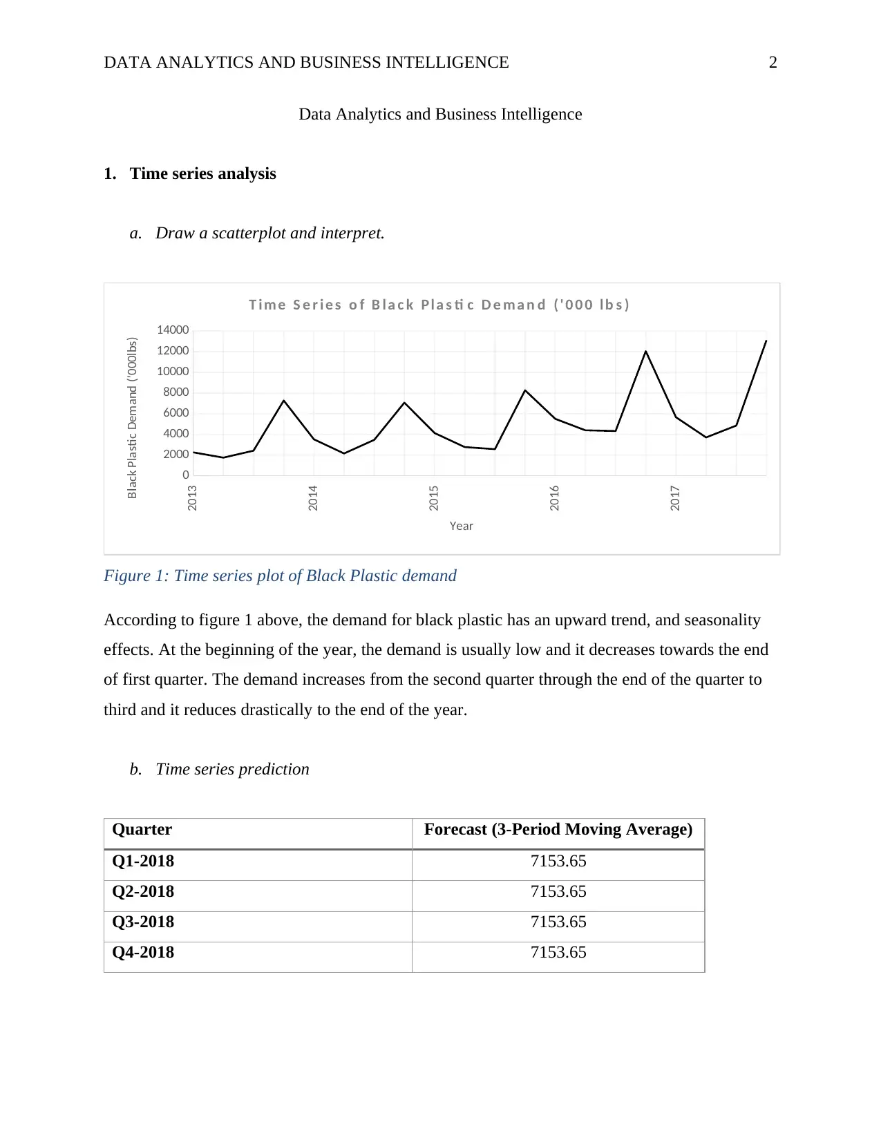
Figure 1: Time series plot of Black Plastic demand
According to figure 1 above, the demand for black plastic has an upward trend, and seasonality
effects. At the beginning of the year, the demand is usually low and it decreases towards the end
of first quarter. The demand increases from the second quarter through the end of the quarter to
third and it reduces drastically to the end of the year.
b. Time series prediction
Quarter Forecast (3-Period Moving Average)
Q1-2018 7153.65
Q2-2018 7153.65
Q3-2018 7153.65
Q4-2018 7153.65

DATA ANALYTICS AND BUSINESS INTELLIGENCE 3
Q1-2013
Q2-2013
Q3-2013
Q4-2013
Q1-2014
Q2-2014
Q3-2014
Q4-2014
Q1-2015
Q2-2015
Q3-2015
Q4-2015
Q1-2016
Q2-2016
Q3-2016
Q4-2016
Q1-2017
Q2-2017
Q3-2017
Q4-2017
Q1-2018
Q2-2018
Q3-2018
Q4-2018
0.00
2000.00
4000.00
6000.00
8000.00
10000.00
12000.00
14000.00
Forecast and Original Observations
Black Plastic Demand ('000 lbs) Forecast
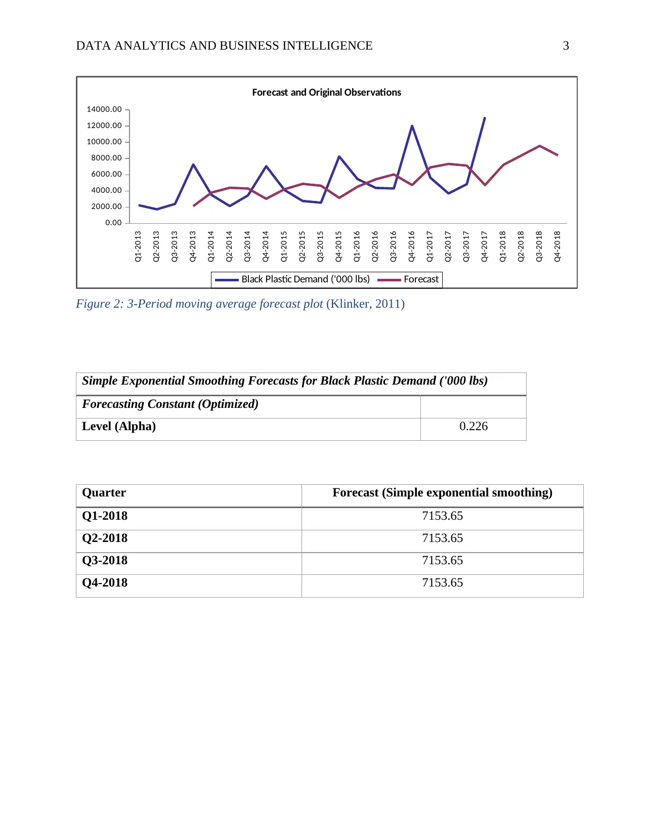
Figure 2: 3-Period moving average forecast plot (Klinker, 2011)
Simple Exponential Smoothing Forecasts for Black Plastic Demand ('000 lbs)
Forecasting Constant (Optimized)
Level (Alpha) 0.226
Quarter Forecast (Simple exponential smoothing)
Q1-2018 7153.65
Q2-2018 7153.65
Q3-2018 7153.65
Q4-2018 7153.65

DATA ANALYTICS AND BUSINESS INTELLIGENCE 4
Q1-2013
Q2-2013
Q3-2013
Q4-2013
Q1-2014
Q2-2014
Q3-2014
Q4-2014
Q1-2015
Q2-2015
Q3-2015
Q4-2015
Q1-2016
Q2-2016
Q3-2016
Q4-2016
Q1-2017
Q2-2017
Q3-2017
Q4-2017
Q1-2018
Q2-2018
Q3-2018
Q4-2018
0.00
2000.00
4000.00
6000.00
8000.00
10000.00
12000.00
14000.00
Forecast and Original Observations
Black Plastic Demand ('000 lbs) Forecast
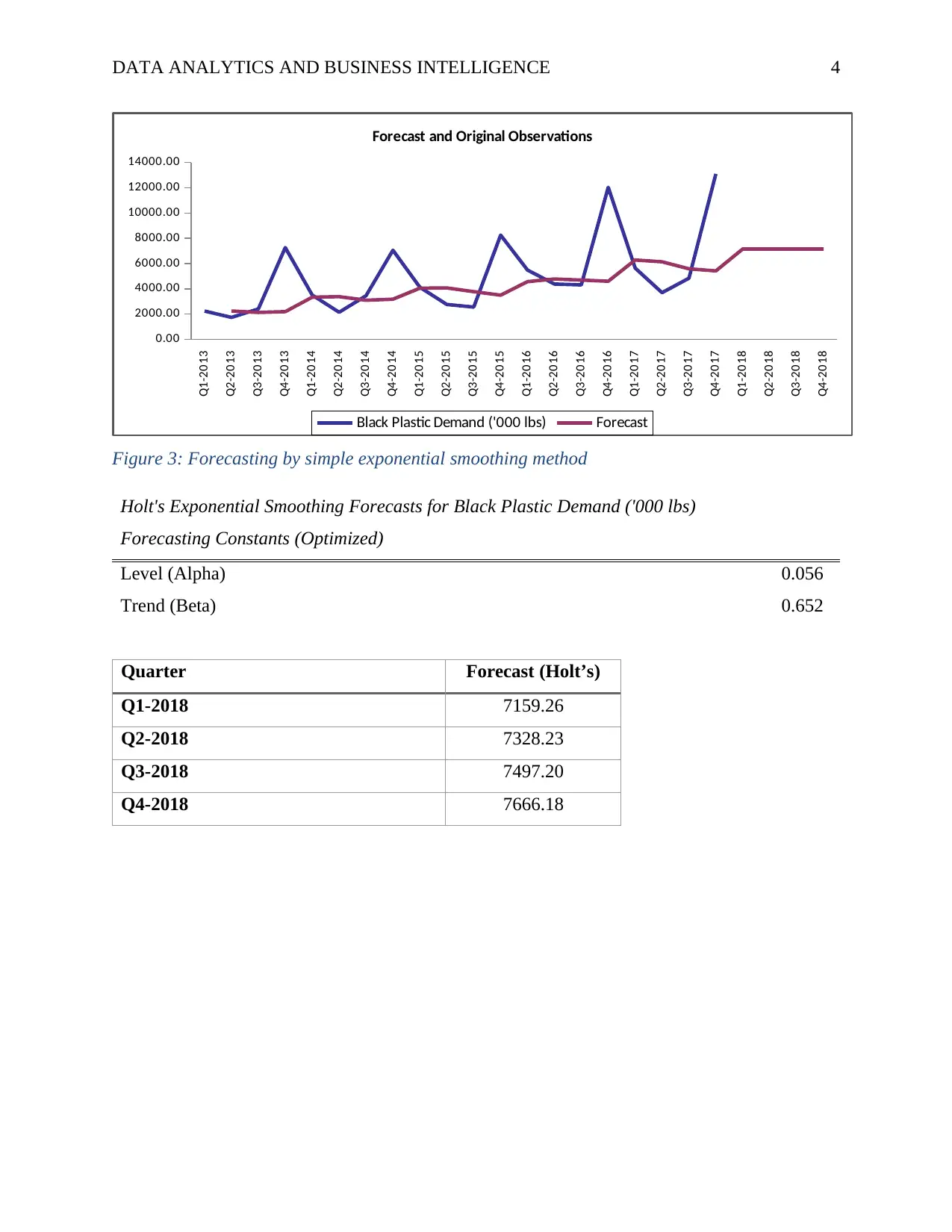
Figure 3: Forecasting by simple exponential smoothing method
Holt's Exponential Smoothing Forecasts for Black Plastic Demand ('000 lbs)
Forecasting Constants (Optimized)
Level (Alpha) 0.056
Trend (Beta) 0.652
Quarter Forecast (Holt’s)
Q1-2018 7159.26
Q2-2018 7328.23
Q3-2018 7497.20
Q4-2018 7666.18

DATA ANALYTICS AND BUSINESS INTELLIGENCE 5
Q1-2013
Q2-2013
Q3-2013
Q4-2013
Q1-2014
Q2-2014
Q3-2014
Q4-2014
Q1-2015
Q2-2015
Q3-2015
Q4-2015
Q1-2016
Q2-2016
Q3-2016
Q4-2016
Q1-2017
Q2-2017
Q3-2017
Q4-2017
Q1-2018
Q2-2018
Q3-2018
Q4-2018
0.00
2000.00
4000.00
6000.00
8000.00
10000.00
12000.00
14000.00
Forecast and Original Observations
Black Plastic Demand ('000 lbs) Forecast
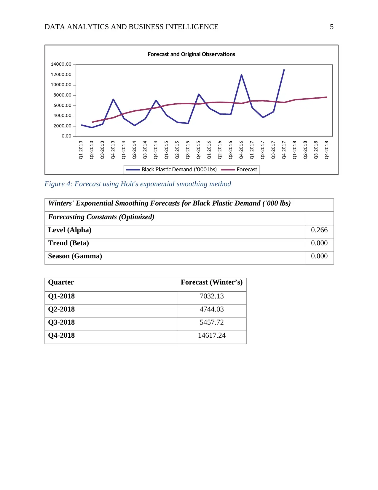
Figure 4: Forecast using Holt's exponential smoothing method
Winters' Exponential Smoothing Forecasts for Black Plastic Demand ('000 lbs)
Forecasting Constants (Optimized)
Level (Alpha) 0.266
Trend (Beta) 0.000
Season (Gamma) 0.000
Quarter Forecast (Winter’s)
Q1-2018 7032.13
Q2-2018 4744.03
Q3-2018 5457.72
Q4-2018 14617.24

DATA ANALYTICS AND BUSINESS INTELLIGENCE 6
Q1-2013
Q2-2013
Q3-2013
Q4-2013
Q1-2014
Q2-2014
Q3-2014
Q4-2014
Q1-2015
Q2-2015
Q3-2015
Q4-2015
Q1-2016
Q2-2016
Q3-2016
Q4-2016
Q1-2017
Q2-2017
Q3-2017
Q4-2017
Q1-2018
Q2-2018
Q3-2018
Q4-2018
0.00
2000.00
4000.00
6000.00
8000.00
10000.00
12000.00
14000.00
16000.00
Forecast and Original Observations
Black Plastic Demand ('000 lbs) Forecast
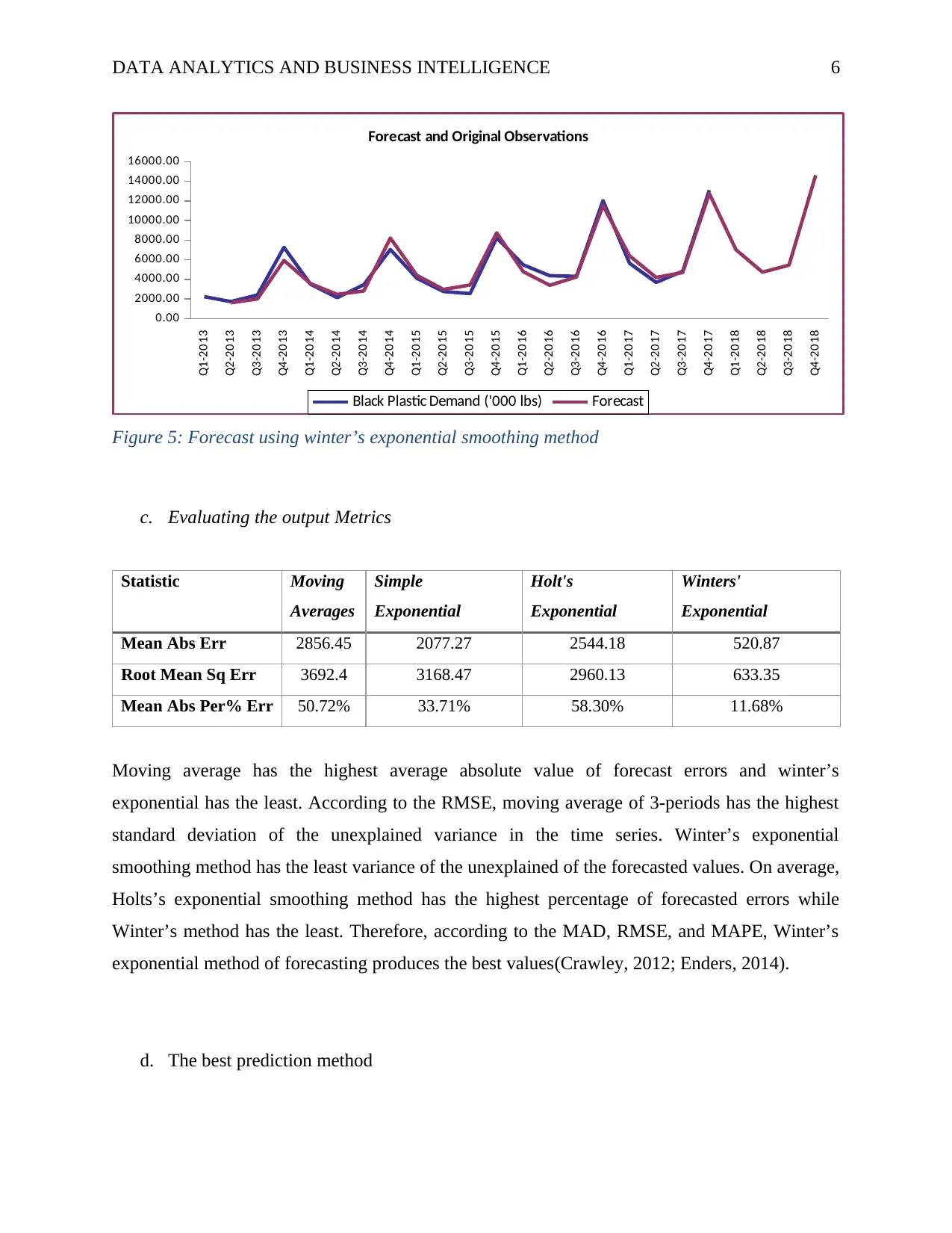
Figure 5: Forecast using winter’s exponential smoothing method
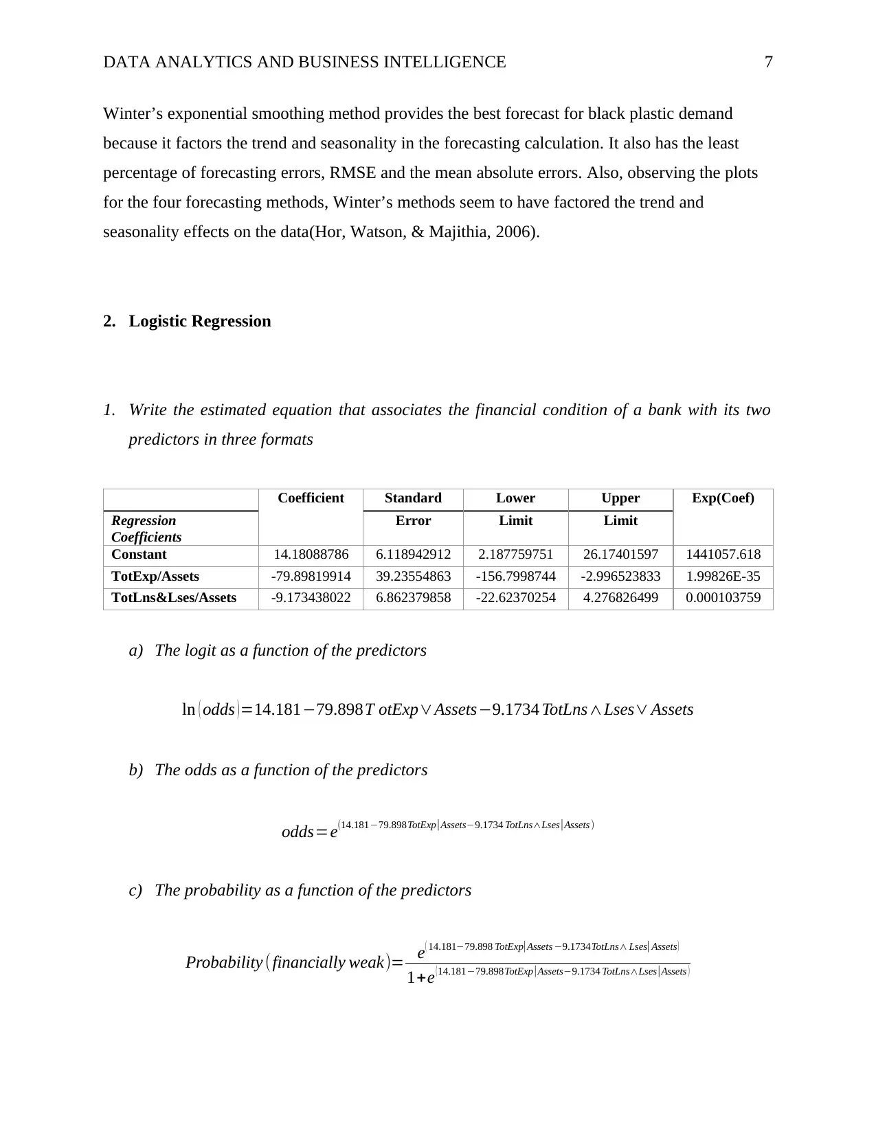
c. Evaluating the output Metrics
Statistic Moving
Averages
Simple
Exponential
Holt's
Exponential
Winters'
Exponential
Mean Abs Err 2856.45 2077.27 2544.18 520.87
Root Mean Sq Err 3692.4 3168.47 2960.13 633.35
Mean Abs Per% Err 50.72% 33.71% 58.30% 11.68%
Moving average has the highest average absolute value of forecast errors and winter’s
exponential has the least. According to the RMSE, moving average of 3-periods has the highest
standard deviation of the unexplained variance in the time series. Winter’s exponential
smoothing method has the least variance of the unexplained of the forecasted values. On average,
Holts’s exponential smoothing method has the highest percentage of forecasted errors while
Winter’s method has the least. Therefore, according to the MAD, RMSE, and MAPE, Winter’s
exponential method of forecasting produces the best values(Crawley, 2012; Enders, 2014).
d. The best prediction method

DATA ANALYTICS AND BUSINESS INTELLIGENCE 7
Winter’s exponential smoothing method provides the best forecast for black plastic demand
because it factors the trend and seasonality in the forecasting calculation. It also has the least
percentage of forecasting errors, RMSE and the mean absolute errors. Also, observing the plots
for the four forecasting methods, Winter’s methods seem to have factored the trend and
seasonality effects on the data(Hor, Watson, & Majithia, 2006).
2. Logistic Regression
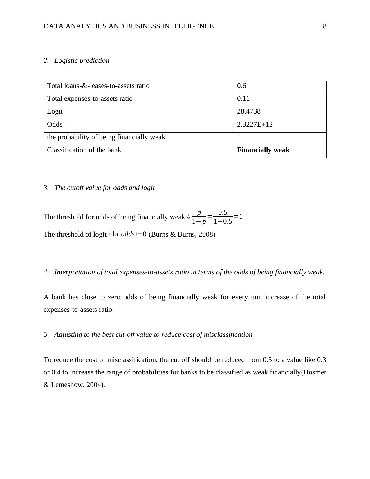
1. Write the estimated equation that associates the financial condition of a bank with its two
predictors in three formats
Coefficient Standard Lower Upper Exp(Coef)
Regression
Coefficients
Error Limit Limit
Constant 14.18088786 6.118942912 2.187759751 26.17401597 1441057.618
TotExp/Assets -79.89819914 39.23554863 -156.7998744 -2.996523833 1.99826E-35
TotLns&Lses/Assets -9.173438022 6.862379858 -22.62370254 4.276826499 0.000103759
a) The logit as a function of the predictors
ln ( odds ) =14.181−79.898T otExp∨Assets−9.1734 TotLns∧Lses∨ Assets
b) The odds as a function of the predictors
odds=e(14.181−79.898TotExp |Assets−9.1734 TotLns∧Lses |Assets )
c) The probability as a function of the predictors
Probability (financially weak)= e( 14.181−79.898 TotExp| Assets −9.1734TotLns∧ Lses| Assets )
1+e ( 14.181−79.898TotExp | Assets−9.1734 TotLns∧Lses| Assets )

DATA ANALYTICS AND BUSINESS INTELLIGENCE 8
2. Logistic prediction
Total loans-&-leases-to-assets ratio 0.6
Total expenses-to-assets ratio 0.11
Logit 28.4738
Odds 2.3227E+12
the probability of being financially weak 1
Classification of the bank Financially weak
3. The cutoff value for odds and logit
The threshold for odds of being financially weak ¿ p
1− p = 0.5
1−0.5 =1
The threshold of logit ¿ ln ( odds )=0 (Burns & Burns, 2008)
4. Interpretation of total expenses-to-assets ratio in terms of the odds of being financially weak.
A bank has close to zero odds of being financially weak for every unit increase of the total
expenses-to-assets ratio.
5. Adjusting to the best cut-off value to reduce cost of misclassification
To reduce the cost of misclassification, the cut off should be reduced from 0.5 to a value like 0.3
or 0.4 to increase the range of probabilities for banks to be classified as weak financially(Hosmer
& Lemeshow, 2004).

DATA ANALYTICS AND BUSINESS INTELLIGENCE 9
References
Burns, R. P., & Burns, R. (2008). Chapter 24 Logistic Regression. Business Research Methods
and Statistics Using SPSS, (Chapter 25), 344–354. Retrieved from
http://books.google.com/books?
hl=en&lr=&id=bPvCRzBou3gC&oi=fnd&pg=PR5&dq=Business+
Research+Methods+and+Statistics+using+SPSS&ots=evyQoeCAur&sig=oR9vX
qT9KivGjvQzYZFufAWO5bU
Crawley, M. J. (2012). Time Series Analysis. The R Book, 785–808.
https://doi.org/10.1002/9781118448908.ch24
Enders, W. (2014). Applied Econometric Time Series. Technometrics (Vol. 46).
https://doi.org/10.1198/tech.2004.s813
Hor, C.-L., Watson, S. J., & Majithia, S. (2006). Time series analysis. Transmission and
Distribution (Former Title), 142(3), 614. https://doi.org/10.1007/SpringerReference_6246
Hosmer, D. W., & Lemeshow, S. (2004). Applied Logistic Regression Second Edition. Applied
Logistic Regression. https://doi.org/10.1002/0471722146
Klinker, F. (2011). Exponential moving average versus moving exponential average.
Mathematische Semesterberichte, 58(1), 97–107. https://doi.org/10.1007/s00591-010-0080-

DATA ANALYTICS AND BUSINESS INTELLIGENCE 10
8