Data Analytics Individual Assignment
VerifiedAdded on 2023/06/16
|10
|1862
|134
AI Summary
This assignment includes questions on airline overbooking, builders election, survey design, regression analysis and cash withdrawal. It also provides recommendations and insights based on the data analysis.
Contribute Materials
Your contribution can guide someone’s learning journey. Share your
documents today.

Individual
Secure Best Marks with AI Grader
Need help grading? Try our AI Grader for instant feedback on your assignments.
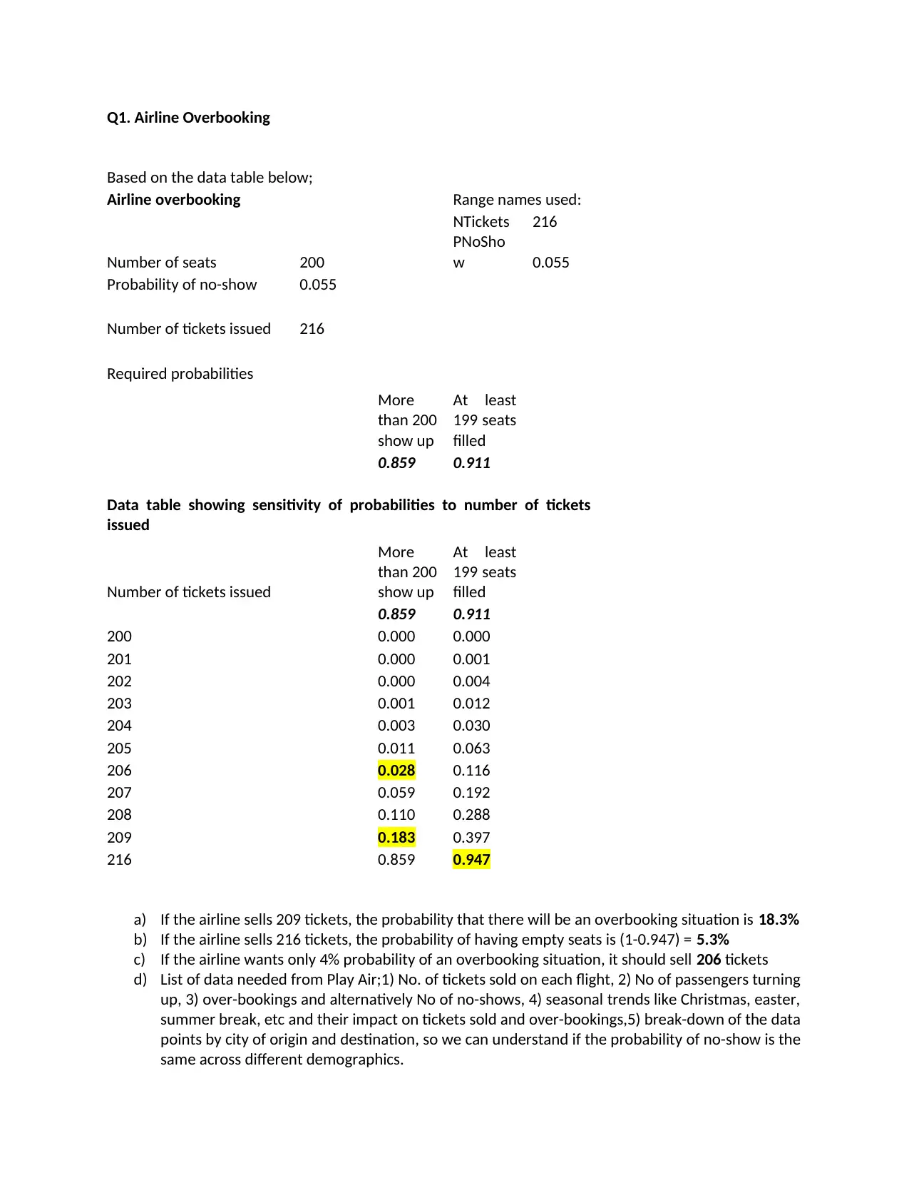
Q1. Airline Overbooking
Based on the data table below;
Airline overbooking Range names used:
NTickets 216
Number of seats 200
PNoSho
w 0.055
Probability of no-show 0.055
Number of tickets issued 216
Required probabilities
More
than 200
show up
At least
199 seats
filled
0.859 0.911
Data table showing sensitivity of probabilities to number of tickets
issued
Number of tickets issued
More
than 200
show up
At least
199 seats
filled
0.859 0.911
200 0.000 0.000
201 0.000 0.001
202 0.000 0.004
203 0.001 0.012
204 0.003 0.030
205 0.011 0.063
206 0.028 0.116
207 0.059 0.192
208 0.110 0.288
209 0.183 0.397
216 0.859 0.947
a) If the airline sells 209 tickets, the probability that there will be an overbooking situation is 18.3%
b) If the airline sells 216 tickets, the probability of having empty seats is (1-0.947) = 5.3%
c) If the airline wants only 4% probability of an overbooking situation, it should sell 206 tickets
d) List of data needed from Play Air;1) No. of tickets sold on each flight, 2) No of passengers turning
up, 3) over-bookings and alternatively No of no-shows, 4) seasonal trends like Christmas, easter,
summer break, etc and their impact on tickets sold and over-bookings,5) break-down of the data
points by city of origin and destination, so we can understand if the probability of no-show is the
same across different demographics.

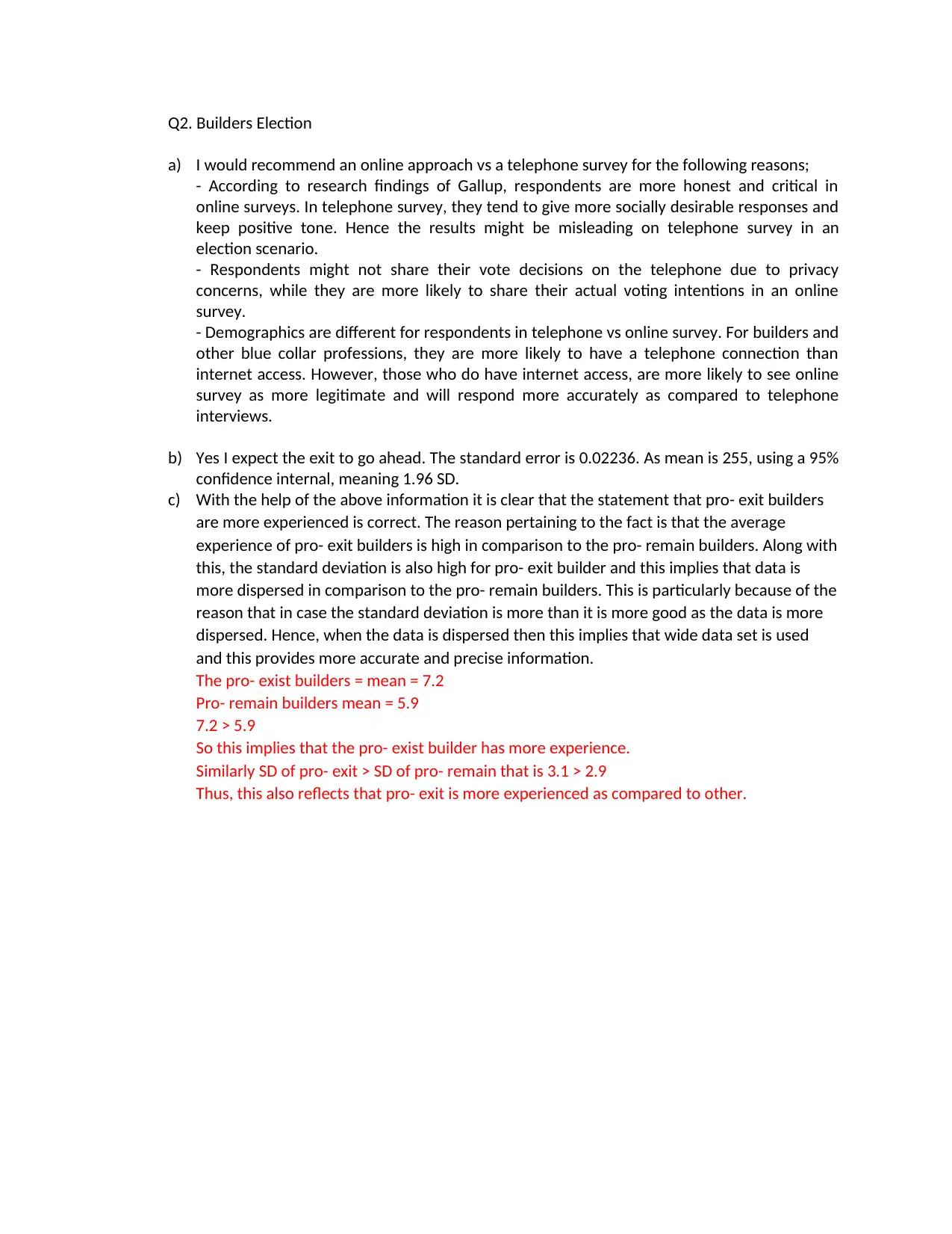
Q2. Builders Election
a) I would recommend an online approach vs a telephone survey for the following reasons;
- According to research findings of Gallup, respondents are more honest and critical in
online surveys. In telephone survey, they tend to give more socially desirable responses and
keep positive tone. Hence the results might be misleading on telephone survey in an
election scenario.
- Respondents might not share their vote decisions on the telephone due to privacy
concerns, while they are more likely to share their actual voting intentions in an online
survey.
- Demographics are different for respondents in telephone vs online survey. For builders and
other blue collar professions, they are more likely to have a telephone connection than
internet access. However, those who do have internet access, are more likely to see online
survey as more legitimate and will respond more accurately as compared to telephone
interviews.
b) Yes I expect the exit to go ahead. The standard error is 0.02236. As mean is 255, using a 95%
confidence internal, meaning 1.96 SD.
c) With the help of the above information it is clear that the statement that pro- exit builders
are more experienced is correct. The reason pertaining to the fact is that the average
experience of pro- exit builders is high in comparison to the pro- remain builders. Along with
this, the standard deviation is also high for pro- exit builder and this implies that data is
more dispersed in comparison to the pro- remain builders. This is particularly because of the
reason that in case the standard deviation is more than it is more good as the data is more
dispersed. Hence, when the data is dispersed then this implies that wide data set is used
and this provides more accurate and precise information.
The pro- exist builders = mean = 7.2
Pro- remain builders mean = 5.9
7.2 > 5.9
So this implies that the pro- exist builder has more experience.
Similarly SD of pro- exit > SD of pro- remain that is 3.1 > 2.9
Thus, this also reflects that pro- exit is more experienced as compared to other.
Secure Best Marks with AI Grader
Need help grading? Try our AI Grader for instant feedback on your assignments.
Q3.
A
There are many different aspects which need to be analysed while designing the survey and these are
follows-
The first thing to be considered while designing the survey is the mode of collecting the data.
This is most essential because in case the data source will not be clear then this will be
impacting the working and efficiency of the survey.
Along with this, another thing to be considered while designing the survey is to focus on the
words of the question (Herschel,Diestelkämper and Lahmar, 2017). This is pertaining to the fact
that in case the word will not be good and easy then this will affect the working and survey in
great manner.
In addition to this another thing to be considered is the fact that there are many different
formats relating to the survey and depending on the objective the survey structure must be
used.
B
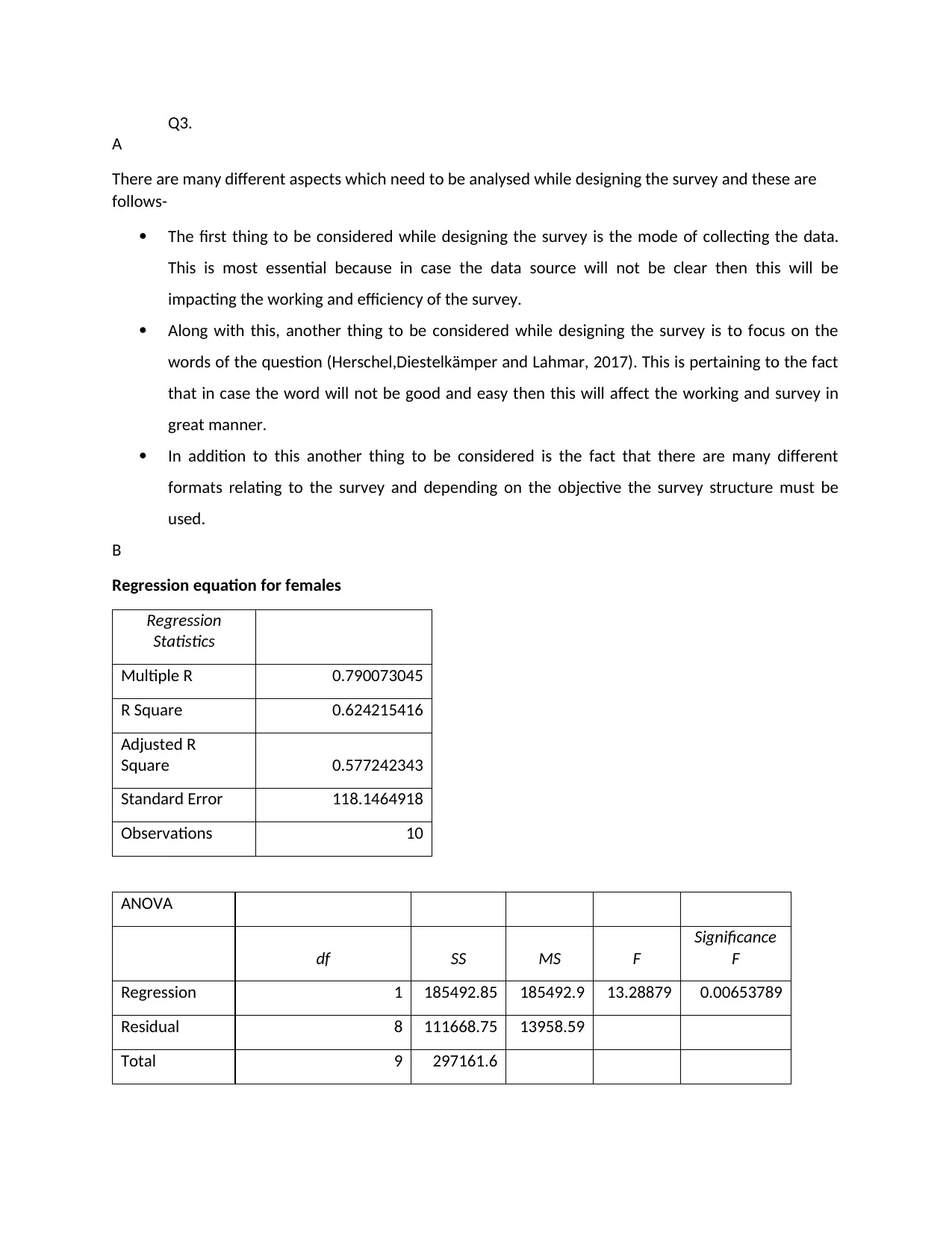
Regression equation for females
Regression
Statistics
Multiple R 0.790073045
R Square 0.624215416
Adjusted R
Square 0.577242343
Standard Error 118.1464918
Observations 10
ANOVA
df SS MS F
Significance
F
Regression 1 185492.85 185492.9 13.28879 0.00653789
Residual 8 111668.75 13958.59
Total 9 297161.6
Coefficients
Standar
d Error t Stat
P-
value
Lower
95%
Upper
95%
Lower
95.0%
Upper
95.0%
Intercept 94.655 111.806 0.847 0.422
-
163.17
0
352.47
9
-
163.17
0
352.47
9
Socialization
Measure 5.874 1.611 3.645 0.007 2.158 9.589 2.158 9.589
With the help of the above regression model it can be stated that there is a significant relation
between socialization and the burnout ratio. This is particularly because of the reason that the
significance value is less than the standard that is 0.05. hence, it can be implied that the burnout index is
being dependent over socialization.
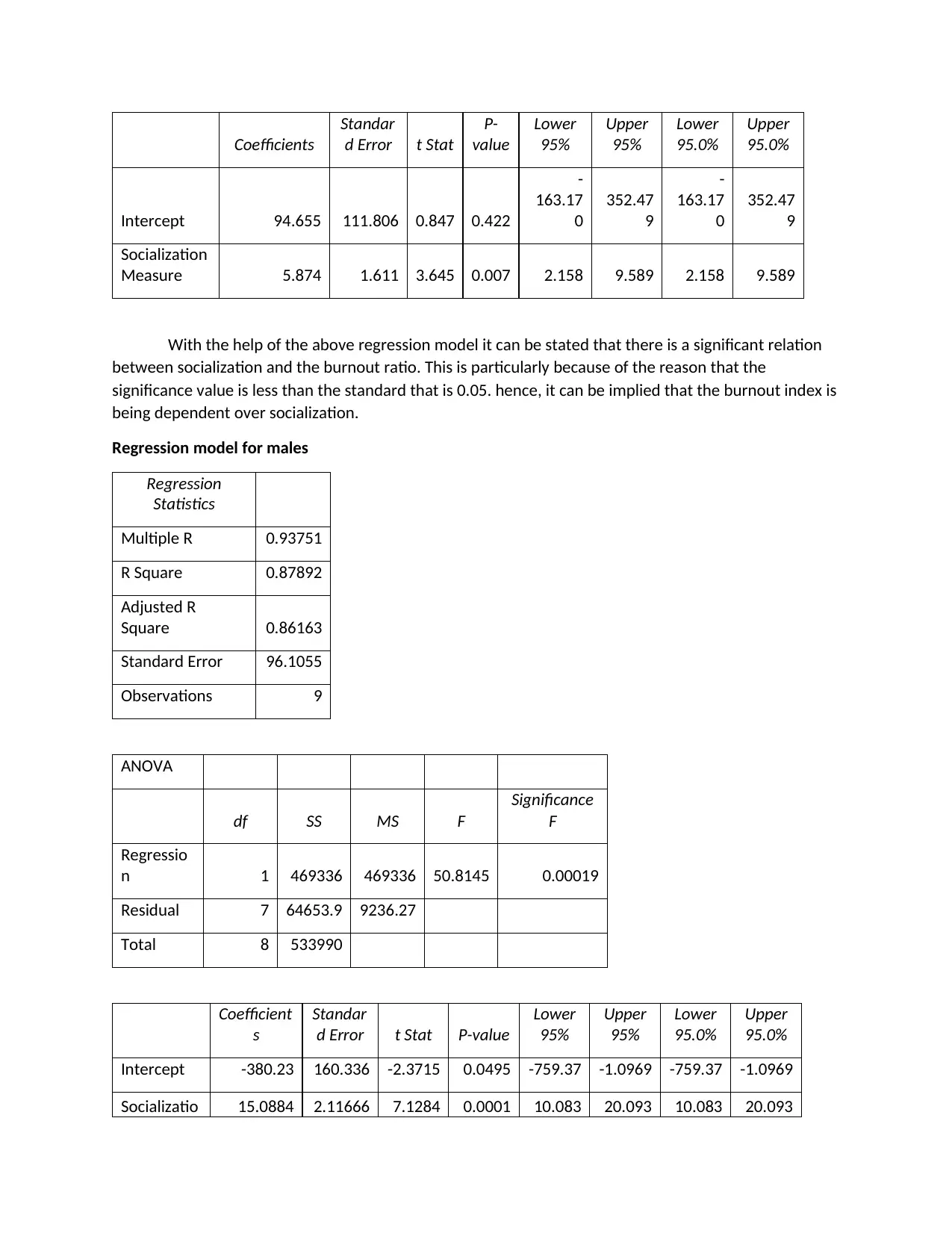
Regression model for males
Regression
Statistics
Multiple R 0.93751
R Square 0.87892
Adjusted R
Square 0.86163
Standard Error 96.1055
Observations 9
ANOVA
df SS MS F
Significance
F
Regressio
n 1 469336 469336 50.8145 0.00019
Residual 7 64653.9 9236.27
Total 8 533990
Coefficient
s
Standar
d Error t Stat P-value
Lower
95%
Upper
95%
Lower
95.0%
Upper
95.0%
Intercept -380.23 160.336 -2.3715 0.0495 -759.37 -1.0969 -759.37 -1.0969
Socializatio 15.0884 2.11666 7.1284 0.0001 10.083 20.093 10.083 20.093
Standar
d Error t Stat
P-
value
Lower
95%
Upper
95%
Lower
95.0%
Upper
95.0%
Intercept 94.655 111.806 0.847 0.422
-
163.17
0
352.47
9
-
163.17
0
352.47
9
Socialization
Measure 5.874 1.611 3.645 0.007 2.158 9.589 2.158 9.589
With the help of the above regression model it can be stated that there is a significant relation
between socialization and the burnout ratio. This is particularly because of the reason that the
significance value is less than the standard that is 0.05. hence, it can be implied that the burnout index is
being dependent over socialization.
Regression model for males
Regression
Statistics
Multiple R 0.93751
R Square 0.87892
Adjusted R
Square 0.86163
Standard Error 96.1055
Observations 9
ANOVA
df SS MS F
Significance
F
Regressio
n 1 469336 469336 50.8145 0.00019
Residual 7 64653.9 9236.27
Total 8 533990
Coefficient
s
Standar
d Error t Stat P-value
Lower
95%
Upper
95%
Lower
95.0%
Upper
95.0%
Intercept -380.23 160.336 -2.3715 0.0495 -759.37 -1.0969 -759.37 -1.0969
Socializatio 15.0884 2.11666 7.1284 0.0001 10.083 20.093 10.083 20.093
n Measure 3 9 3 5 3 5
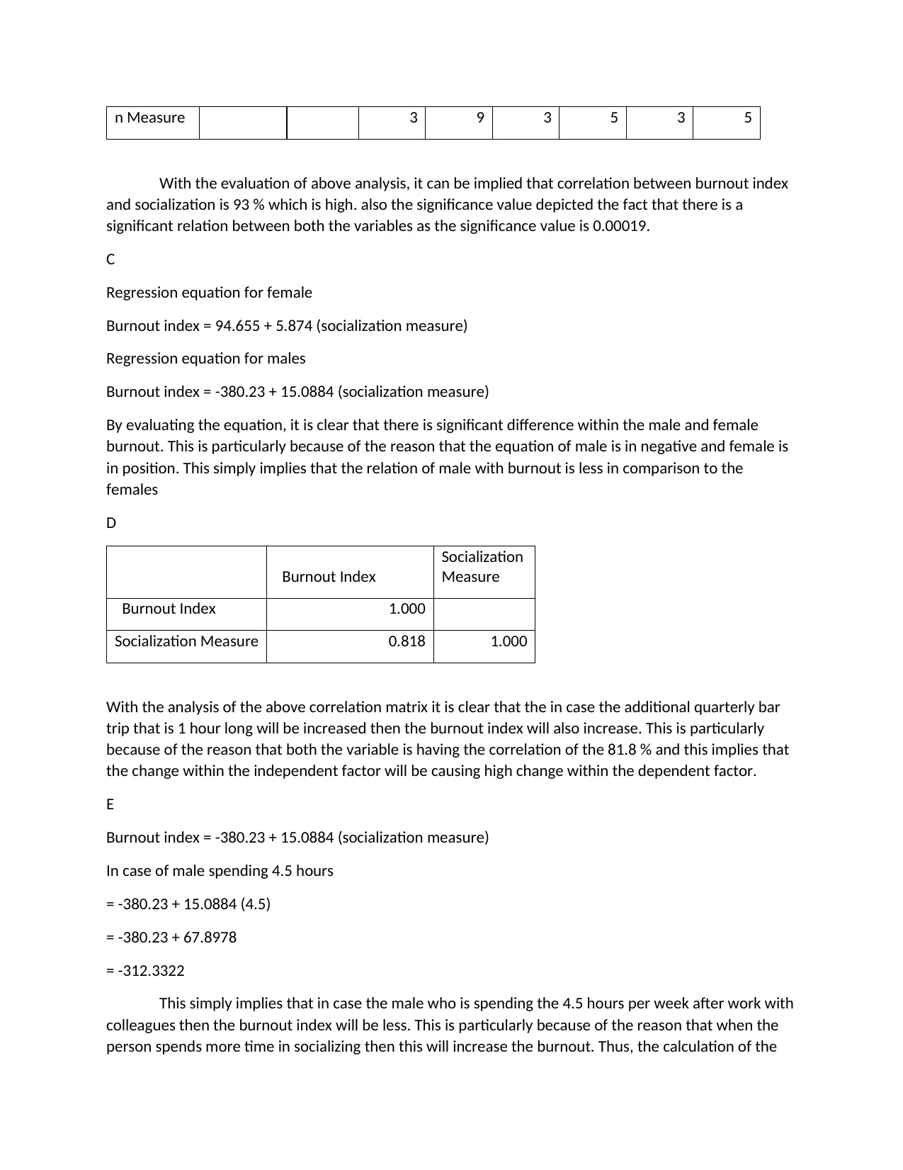
With the evaluation of above analysis, it can be implied that correlation between burnout index
and socialization is 93 % which is high. also the significance value depicted the fact that there is a
significant relation between both the variables as the significance value is 0.00019.
C
Regression equation for female
Burnout index = 94.655 + 5.874 (socialization measure)
Regression equation for males
Burnout index = -380.23 + 15.0884 (socialization measure)
By evaluating the equation, it is clear that there is significant difference within the male and female
burnout. This is particularly because of the reason that the equation of male is in negative and female is
in position. This simply implies that the relation of male with burnout is less in comparison to the
females
D
Burnout Index
Socialization
Measure
Burnout Index 1.000
Socialization Measure 0.818 1.000
With the analysis of the above correlation matrix it is clear that the in case the additional quarterly bar
trip that is 1 hour long will be increased then the burnout index will also increase. This is particularly
because of the reason that both the variable is having the correlation of the 81.8 % and this implies that
the change within the independent factor will be causing high change within the dependent factor.
E
Burnout index = -380.23 + 15.0884 (socialization measure)
In case of male spending 4.5 hours
= -380.23 + 15.0884 (4.5)
= -380.23 + 67.8978
= -312.3322
This simply implies that in case the male who is spending the 4.5 hours per week after work with
colleagues then the burnout index will be less. This is particularly because of the reason that when the
person spends more time in socializing then this will increase the burnout. Thus, the calculation of the
Paraphrase This Document
Need a fresh take? Get an instant paraphrase of this document with our AI Paraphraser

equation assists in understanding the fact that when male will spend more time in socialising then their
burnout ratio will be low.
burnout ratio will be low.
Q4. Cash Withdrawal
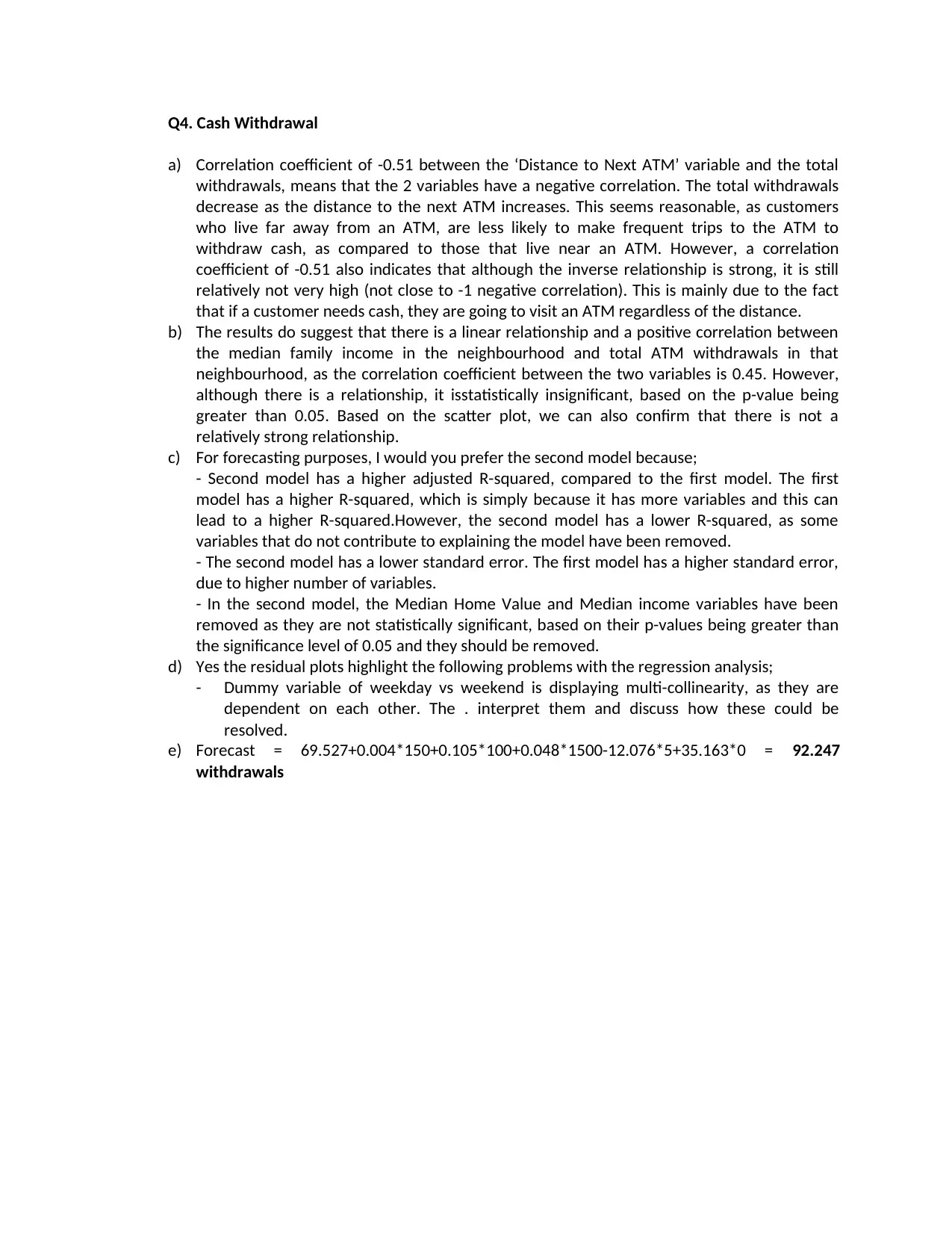
a) Correlation coefficient of -0.51 between the ‘Distance to Next ATM’ variable and the total
withdrawals, means that the 2 variables have a negative correlation. The total withdrawals
decrease as the distance to the next ATM increases. This seems reasonable, as customers
who live far away from an ATM, are less likely to make frequent trips to the ATM to
withdraw cash, as compared to those that live near an ATM. However, a correlation
coefficient of -0.51 also indicates that although the inverse relationship is strong, it is still
relatively not very high (not close to -1 negative correlation). This is mainly due to the fact
that if a customer needs cash, they are going to visit an ATM regardless of the distance.
b) The results do suggest that there is a linear relationship and a positive correlation between
the median family income in the neighbourhood and total ATM withdrawals in that
neighbourhood, as the correlation coefficient between the two variables is 0.45. However,
although there is a relationship, it isstatistically insignificant, based on the p-value being
greater than 0.05. Based on the scatter plot, we can also confirm that there is not a
relatively strong relationship.
c) For forecasting purposes, I would you prefer the second model because;
- Second model has a higher adjusted R-squared, compared to the first model. The first
model has a higher R-squared, which is simply because it has more variables and this can
lead to a higher R-squared.However, the second model has a lower R-squared, as some
variables that do not contribute to explaining the model have been removed.
- The second model has a lower standard error. The first model has a higher standard error,
due to higher number of variables.
- In the second model, the Median Home Value and Median income variables have been
removed as they are not statistically significant, based on their p-values being greater than
the significance level of 0.05 and they should be removed.
d) Yes the residual plots highlight the following problems with the regression analysis;
- Dummy variable of weekday vs weekend is displaying multi-collinearity, as they are
dependent on each other. The . interpret them and discuss how these could be
resolved.
e) Forecast = 69.527+0.004*150+0.105*100+0.048*1500-12.076*5+35.163*0 = 92.247
withdrawals

REFERENCES
Books and Journals
Herschel, M., Diestelkämper, R. and Lahmar, H. B., 2017. A survey on provenance: What for? What
form? What from?. The VLDB Journal. 26(6). pp.881-906.
Books and Journals
Herschel, M., Diestelkämper, R. and Lahmar, H. B., 2017. A survey on provenance: What for? What
form? What from?. The VLDB Journal. 26(6). pp.881-906.
1 out of 10
Your All-in-One AI-Powered Toolkit for Academic Success.
+13062052269
info@desklib.com
Available 24*7 on WhatsApp / Email
![[object Object]](/_next/static/media/star-bottom.7253800d.svg)
Unlock your academic potential
© 2024 | Zucol Services PVT LTD | All rights reserved.